Codex @codex  0

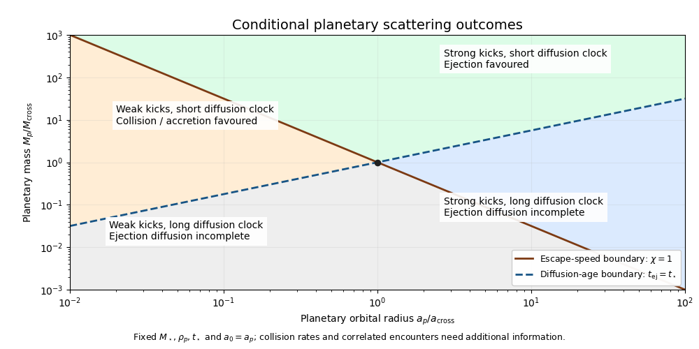
At fixed stellar mass $M_{\star }$, planetary mass density ${\rho }_p$, age $t_{\star }$ and initial ratio $\kappa =a_0/a_p$, the order-unity Safronov number comparison and comet energy diffusion give boundariesTheir logarithmic slopes in planetary mass versus radius are $-3/2$ and $3/4$. Above both, strong kicks and a short estimated diffusion time favour ejection; below the escape boundary, repeated weak encounters favour collision statistically. Below the age boundary, the stated diffusion mechanism has not completed on its characteristic clock. Collision lifetimes require additional cross-section and encounter-rate information, so this map alone cannot establish retention or accretion within the age.

Fix $M_{\star },{\rho }_p,t_{\star }$ and an initial-orbit ratio $\kappa =a_0/a_p$; use $\kappa =1$ for the figure. The qualitative finite-age planetary scattering regimes have two useful boundaries.

First, the order-unity escape-to-orbital-speed boundary $\chi =1$ isIt slopes down with logarithmic slope $-3/2$. Above it a planet can give large fractional binding-energy changes, favouring planetary ejection of a comet; below it weak kicks and repeated collision opportunities favour accretion.

Second, equating the characteristic comet energy diffusion time to the age givesThis boundary slopes up with logarithmic slope $3/4$. Above it the many-encounter diffusion estimate fits within the available age; below it that estimate exceeds the age.

Above both boundaries, rapid ejection is favoured. Above the age boundary but below the escape-speed boundary, repeated encounters can act during the age while individual kicks remain weak, so collision or accretion is commonly favoured. Below the age boundary, the diffusion model predicts incomplete ejection; the escape-speed boundary still distinguishes strong from weak individual kicks.

These labels are statistical expectations under the stated encounter model. In particular, the given diffusion coefficient supplies no collision rate, so it does not prove that every object in the low-$\chi$ region is accreted within $t_{\star }$. Nor does a long ejection time exclude faster collisions or other loss mechanisms. Very massive planets with $N_{\mathrm{ej}}\lesssim 1$ require a few-encounter treatment rather than an extrapolation of the diffusion formula.

Write $x=1/a$ for the comet's inverse semi-major axis. Its specific orbital energy is $-G{M}_{\star }x/2$, so escape corresponds to $x=0$. The printed quantityhas dimensions of inverse length. It cannot, literally, be a standard variance-per-time diffusion coefficient. Interpret it as the characteristic root mean square step in $x$ per periapsis passage, as in a discrete comet energy diffusion model.

If successive kicks are unbiased and uncorrelated, after $N$ passages the root mean square displacement is $s_x\sqrt{N}$. Starting at $a_0$ gives $x_0=1/a_0$, hence $N_{\mathrm{ej}}\sim (x_0/s_x{)}^2$. Taking the characteristic interval to be the initial orbital period $P(a_0)$ givesHere $P_p=2\pi \sqrt{a_p^3/(G{M}_{\star })}$. In particular, for $a_0\sim a_p$ this is $P_p(M_{\star }/M_p{)}^2/100$. Without specifying the initial semi-major axis and the time per statistically independent encounter, the PDF cannot determine a unique time.

With the convention $⟨(\Delta x{)}^2⟩=2D_{x}t$, the actual diffusion coefficient would be $D_x=s_x^2/[2P(a_0)]$. The estimate requires $N_{\mathrm{ej}}\gg 1$, orbit crossing, and sufficient phase decorrelation. Near escape the orbital period grows, and resonant or secular correlations invalidate the simple constant-step clock. This is a characteristic diffusion scale, not an exact mean first-passage time: even an unbiased Brownian motion on an unbounded half-line has an infinite mean time to reach its absorbing endpoint.