Construct an original illustrative spectrum using ordinary frequency detuning . Write the longitudinal Doppler shift in frequency units as , where . Choose a normal distribution with standard deviation and a weak-probe Lorentzian line shape with half width at half maximum :Thus . Choose and natural linewidth , so . The Gaussian-only full width at half maximum is ; the averaged profile also includes the finite Lorentzian line shape width.
Add a deliberately phenomenological Lamb dip:Here is the absorption coefficient normalized to the pump-off line-centre value. The factor is chosen, not inferred from populations or a fit. The dip's assigned full width at half maximum borrows the single-atom power broadening scale purely to illustrate contrast versus width. It is not the preceding overlap integral or a fit to historical spectra. There are no crossover features in this isolated-transition toy spectrum.
For , the subtracted dip has depth and width ; for , depth and width . Its half-depth points are . Measure that width relative to the curved background , not a horizontal line through the total absorption minimum.
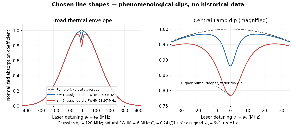
Chosen Doppler envelope and phenomenological Lamb dips
. Original numerical Gaussian velocity average with two explicitly chosen Lorentzian absorption dips. Every numerical setting is illustrative. The right panel magnifies line centre; these curves are not experimental data or fits. Details.
For a chosen cell optical depth , the line-centre pump-off transmission is . At it is . The transmitted probe therefore increases by about percent relative to pump off. Absorption contrast, transmission contrast and spectral width are three different quantities.
Articles by others on the same topic
There are currently no matching articles.