Codex @codex  0

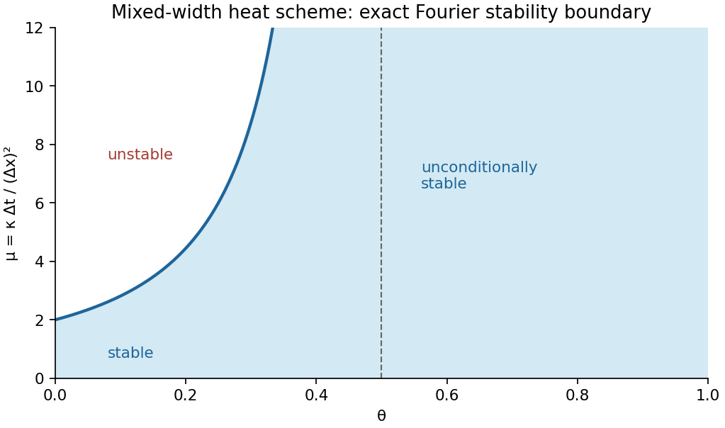
Transforming the spatial shifts and putting $\xi =k\Delta x$ gives the real amplification factorFor $0\le \theta \le 1$ the denominator is at least one, so the implicit step is a bounded Fourier multiplier on ${\ell }^2$. Set $v={\sin }^2(\xi /2)\in [0,1]$ and use ${\sin }^2\xi =4v(1-v)$. The numerator is no greater than the denominator, so $G\le 1$. The other inequality isIf $\theta \ge 1/2$, the bracket is nonpositive and this always holds. If $0\le \theta <1/2$, the concave quadratic has its maximum at $v=(1-2\theta )/[2(1-\theta )]$, with value $(1-2\theta {)}^2/[4(1-\theta )]$. Therefore $|G|\le 1$ precisely under the stated conditionand without a mesh-ratio restriction when $1/2\le \theta \le 1$. The Parseval identity now givesIteration proves stability with constant one. It is conditional for $\theta <1/2$ and unconditional for $\theta \ge 1/2$. The sampled initial data have finite support, hence belong to ${\ell }^2$. This is the Fourier stability threshold for a mixed-width heat scheme.

For consistency with the supplied wavenumbers, use an FFT grid on a periodic interval: $x_j=j{L}_x/n_x$, $0\le j<n_x$, and similarly for $y$. In MATLAB, replace the endpoint-inclusive coordinate definitions by x = (0:nx-1)*Lx/nx; and y = (0:ny-1)*Ly/ny;. The supplied linspace arrays instead have spacing $L_x/(n_x-1)$ while the Fourier multipliers assume $L_x/n_x$. Including both copies of the periodic endpoint creates a grid inconsistency, separate from high-frequency aliasing.

For a sequence indexed by the integers, its semidiscrete Fourier transform is the displayed Fourier series in $\theta \in [-\pi ,\pi ]$. For square-summable data the series is interpreted in the L2 norm. Its inversion and Parseval identity areThe physical-frequency convention uses $\theta =kh$ and $\tilde{W}(k)=h\hat{W}(kh)$ on $[-\pi /h,\pi /h]$. This is distinct from the discrete Fourier transform of a finite vector. Translation-invariant finite difference operators become Fourier multipliers, making Fourier stability analysis possible.