For constant particle speed and electric charge , in a transparent, linear, nonmagnetic medium with isotropy, the Frank-Tamm formula gives the produced photon density:Set it to zero below threshold. Here is the positive elementary charge, is track length, is vacuum wavelength, and is the fine-structure constant. With SI lengths in metres, the density has units ; multiplying by gives a dimensionless expected count. The explicit SI convention isThese conventions agree.[ref]
To check the convention, start from and . Changing variables uses the positive density Jacobian ; since , the coefficient becomes . No factor of the material refractive index belongs in this Jacobian: is not the in-medium wavelength. Multiplication by gives the corresponding energy loss density in this SI nonmagnetic convention:
For an original constant-index example, stipulate , , and . Integration from to givesThus a stipulated track produces about photons in this band in the ideal model. This is an emitted count before absorption, collection losses and detector response, not a brightness measurement or a measured water yield.
Choose an original transparent-band model, defined only for :This chosen refractive index is not a fit to water, glass or the historical liquids. It decreases from to approximately , so the threshold increases across the band. For , solving givesOnly emits. Faster particles with and emit throughout this chosen band. The Cherenkov cone angle and the Frank-Tamm formula are both evaluated with the same .
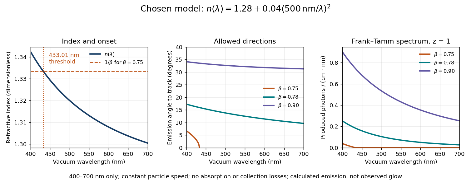
Original dispersive Cherenkov radiation model: a wavelength-dependent threshold, emission angle, and produced photon spectrum
. All curves are calculations for the chosen finite-band refractive index, with and . A missing angular segment means the threshold fails; the corresponding spectral yield is zero. The spectral axis is per centimetre of track and per nanometre of vacuum wavelength, so it is times the density in SI units. No historical observations, measured material constants, absorption or detector response are plotted. Details.For a track the chosen model predicts about , and emitted photons for , and , respectively. An expected count below one is meaningful over repeated equivalent tracks; it is not a fractional photon observed on one track. The near-threshold example illustrates why extending a constant-index approximation across an entire optical band can give the wrong emitting interval.
Finite bandwidth is essential. The factor cannot be extrapolated down to arbitrarily small wavelength: the chosen material model stops at its stated band. Real optical dispersion changes the threshold and direction, and appreciable absorption requires a complex material response beyond the simple transparent-medium expression. A detected count must also include transport, collection geometry and the detector's wavelength-dependent response. Even a correct produced spectrum therefore does not, on its own, predict perceived colour or observed glow intensity.

