The initial table of content was limited to the first level because it is larger than 1000 articles. There are 12823 articles in total. Expand a branch to load its children.
Astrophysics uses physics to explain stars, planets, galaxies, and their electromagnetic radiation; cosmology extends the questions to the universe as a whole. Much of its evidence arrives as light. The challenge is to infer the source's physical properties from what reaches an observer: a bright star might be nearby, unusually luminous, or both. Stellar parallax and observed radiative flux make this distinction quantitative.
This is an inverse problem. A forward problem predicts observations from a source model and the intervening radiative transfer; the inverse problem works backwards from observations to possible models. A spectral line can constrain chemical elements, temperature, and motion through the Doppler effect, but its strength also depends on the stellar atmosphere. Combining different measurements is therefore more informative than interpreting brightness alone. The attraction is that a tiny change in the direction of light can supply a distance, turning received radiative flux into intrinsic luminosity. [ref].
A point-like astronomical source has an angular extent negligible for the calculation or measurement being considered. The ideal mathematical limit concentrates its luminosity at one source-plane position. In gravitational lensing, this approximation permits divergent formal magnifications on a caustic; a finite source averages the magnification over its emitting area. An unresolved source need not have negligible size compared with the lens's caustic scale.
Stellar parallax is the apparent change in a star's viewing direction caused by the observer's changing position. Nearby stars shift more against a distant reference background. In an ideal circular Earth orbit, the conventional annual stellar parallax uses a baseline of one astronomical unit, approximately the Earth-Sun distance. Two opposite observing positions, about six months apart, are separated by approximately two astronomical units. Their maximum angular separation is , so is half that excursion, not the full January-to-July shift. The observed excursion depends on the projected baseline and observing dates. [ref].
For the perpendicular baseline in the diagram, a right triangle giveswhere in the final expression is in radians. Combining the small-angle approximation with the parsec convention givesThus arcseconds implies parsecs, while the ideal six-month excursion is arcseconds. Geometry supplies this distance without assuming a luminosity or a particular stellar atmosphere.
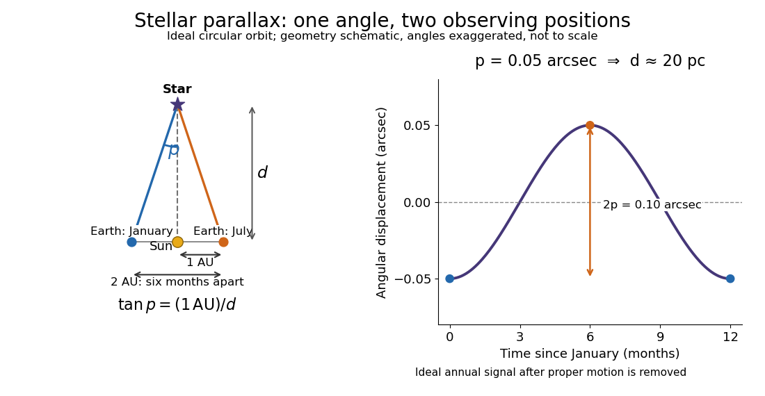
In practical astrometry, many observations separate the annual stellar parallax signal from proper motion, the star's own changing sky position. The Gaia DR3 catalogue reports stellar parallax and its uncertainty in milliarcseconds: arcseconds. A catalogue angle is a fitted measurement with measurement error. [ref].
For a positive stellar parallax with small standard deviation , first-order propagation gives . Thus with gives parsecs with parsecs, assuming systematic offsets are negligible. This linear estimate requires ; a reciprocal is nonlinear and does not generally preserve symmetric uncertainty intervals.
The parsec is a distance unit defined by the exact conventionThe astronomical unit is exactly ; one arcsecond is exactly radians. The IAU resolution explicitly records the parsec convention. A megaparsec is one million parsecs. [ref]. [ref].
The familiar description "the distance giving one arcsecond of stellar parallax" uses the small-angle approximation. Exact right triangle geometry instead gives , slightly shorter than the conventional parsec. The relative difference is approximately . This is negligible for the examples here, but distinguishing an exact unit convention from an approximate geometric interpretation prevents a misleading equality.
The intergalactic medium is the gas between galaxies. Its diffuse, ionized component contains much of the ordinary matter outside stars. Lyman-alpha absorption measures its small neutral-hydrogen fraction, while hotter phases require other tracers.
Diffuse gas in photoionization equilibrium is often approximately described by the displayed temperature-density contrast relation. Photoheating and expansion cooling produce its thermal history. It is an empirical model for low-density gas, not the adiabatic equation of state of every intergalactic phase. Lyman-alpha forest line widths constrain both the temperature at a reference density and the slope through their lower envelope.
The cosmic ionizing background is the diffuse radiation field capable of photoionization of intergalactic gas. Its specific intensity depends on source luminosity functions, ionizing photon escape fractions, cosmological redshifting, and radiative transfer through absorbers. Quasars and star formation supply major contributions with different spectral shapes and evolution.
The Lyman-alpha forest is the multitude of foreground Lyman-alpha absorption features in a distant quasar's spectrum, at wavelengths shorter than its own redshifted Lyman-alpha emission. The quasar supplies a bright background; intervening neutral hydrogen atoms remove photons near their local Lyman-alpha line resonance. Many dips can therefore come from one atomic transition encountered at different redshifts, rather than from many different chemical elements. Some features are instead transitions of other ions, so a dip alone does not identify Lyman-alpha absorption. This makes faint foreground gas detectable through the light it removes, even when its own emission would be difficult to see. [ref]
https://ned.ipac.caltech.edu/level5/Sept01/Rauch/Rauch1.html. Rauch (1998), The Lyman Alpha Forest in the Spectra of QSOs, section 1
.Ignoring peculiar velocity for the moment, an absorber at cosmological redshift puts its Lyman-alpha line atThe rest wavelength is in the ultraviolet; at it appears at in the optical spectrum. In a toy sightline to a quasar at , absorbers at appear at , all shortward of the quasar's Lyman-alpha emission position . The absorbing atoms see the selected photons at their own resonance; the observed dip's redshift belongs to the foreground gas. Peculiar velocity adds a Doppler shift, so the inferred is not a pure distance coordinate. The rest wavelength and resonance interpretation are given in Rauch (1998), section 1.
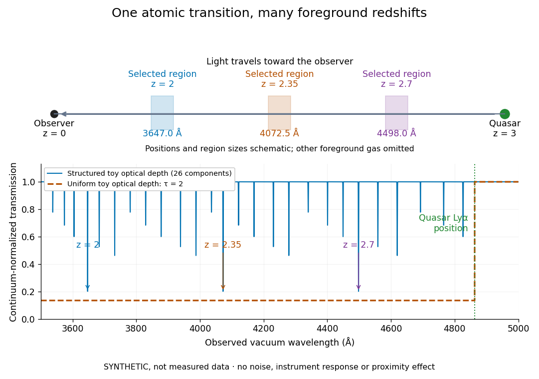
The diagram uses invented optical depths and 26 Doppler cores; three selected foreground regions are marked. Their drawn positions and sizes are schematic. The dashed comparison imposes a uniform optical depth , giving transmission throughout the chosen foreground band. It is an idealized smooth-absorption model, not a measured spectrum or a prediction of the actual intergalactic medium.
The smooth comparison explains the Gunn-Peterson effect: neutral hydrogen distributed throughout an expanding intergalactic medium can absorb continuously over a wavelength interval, because different parts of the path resonate with different observed wavelengths. The resolved Lyman-alpha forest instead has strong transmission fluctuations and distinguishable absorption lines. These need not represent isolated compact clouds: diffuse sheets and filaments in the cosmic web can generate peaks in optical depth along one line of sight. A continuously varying gas distribution can look like a collection of lines. [ref]
https://ned.ipac.caltech.edu/level5/Sept01/Rauch/Rauch1.html. Rauch (1998), section 1: smooth absorption
. [ref]https://ned.ipac.caltech.edu/level5/Sept01/Rauch/Rauch5_1.html. Rauch (1998), section 5.1: synthetic sightlines and extended structures
.An early observation makes the identification concrete. Lynds's 1971 paper analyzed six spectrograms of the quasar 4C 05.34, with emission redshift , taken in spring 1970 using an image-tube spectrograph on Kitt Peak's 84-inch telescope. Five covered – with approximately resolution; the most informative covered about – at resolution. Its reproduced spectrogram shows the strong Lyman-alpha emission flanked mostly on the short-wavelength side by numerous absorption lines. Lynds tabulated their wavelengths and estimated strengths, identified five absorption redshift systems, and proposed that many remaining unidentified lines were the same Lyman-alpha line at additional redshifts. He explicitly warned about blending, an incomplete census of weak lines, and wavelength errors around –. The result established a striking spectral pattern; the paper's proposed interpretation did not measure a separate physical cloud for every dip. [ref]
https://adsabs.harvard.edu/pdf/1971ApJ...164L..73L. Lynds (1971), The Absorption-Line Spectrum of 4C 05.34, Figure 1, Table 1 and discussion
.A contrasting observation demonstrates smooth, very strong absorption. Becker and collaborators (2001) used the Echelle Spectrograph and Imager on Keck II to observe the quasar SDSSp J103027.10+052455.0 at . Sky lines gave an instrumental full width at half maximum of about near , or spectral resolving power . After sky subtraction and flux calibration, the mean continuum-normalized transmission over – was , consistent with zero; this corresponds to absorption redshifts approximately –. They identified a Gunn-Peterson trough. Crucially, resonant Lyman-alpha absorption is so sensitive that even a small neutral fraction can make transmission undetectable: the trough alone does not establish a mostly neutral intergalactic medium or uniquely date reionization. [ref]
https://arxiv.org/pdf/astro-ph/0108097. Becker et al. (2001), sections 2–4: instrument response, transmitted flux and interpretation
.What a spectrum constrains is a radiative transfer problem. For an ideal foreground screen with negligible emission into the observed beam, the intrinsic continuum-normalized transmission isHere is spectral radiative flux, is its unabsorbed continuum, is optical depth, is neutral hydrogen number density, and is neutral hydrogen column density along proper path length . A Voigt profile model constrains redshift, column density and a velocity width together. A nearly black line has lost much of its sensitivity to further increases in optical depth; blending and an uncertain continuum can also admit different fitted components. Finite spectral resolving power and noise limit which widths and weak features can be measured. [ref]
https://ned.ipac.caltech.edu/level5/Sept01/Rauch/Rauch2.html. Rauch (1998), section 2: resolution, noise and profile analysis
. [ref]https://arxiv.org/pdf/astro-ph/0101005. Kim, Cristiani and D'Odorico (2001), section 3: fitted parameters and nonunique profile fits
.For a purely thermal Doppler core, use the velocity convention . The Maxwell-Boltzmann velocity distribution then giveswhere is the Boltzmann constant, is temperature and is a hydrogen atom's mass. This is times the Gaussian distribution's standard deviation. Higher temperature spreads the same column density over more velocities. An instrument also broadens a line: locally, for a nearly flat continuum, the recorded transmission is approximately the convolution of with the normalized instrumental response, not the exponential of a convolved optical depth. A Gaussian response with full width at half maximum has standard deviation , where is the speed of light and the spectral resolving power.
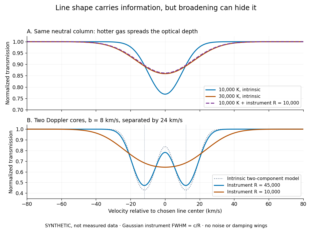
Synthetic absorption profiles: thermal broadening, instrumental smoothing and unresolved blends
. Details. The upper model fixes the integral , hence the neutral hydrogen column density for this transition, while changing temperature. A cooler line blurred by an instrument resembles a warmer intrinsic line. The lower model has two equal Doppler cores separated by : reducing spectral resolving power merges them into one apparent feature. Both panels use invented profiles, Gaussian instrumental responses, and no noise or damping wings. They illustrate an inverse problem, rather than measurements of temperature or a universal relation between a dip and a cloud.
Better observations provide the inputs to that inverse problem. Kim, Cristiani and D'Odorico (2001) analyzed three quasars with the VLT's UVES spectrograph. For HE2217–2818, Table 1 records and of exposure in the – setup in October 1999. Isolated thorium-argon lamp lines measured ; the data were resampled into bins, with signal-to-noise ratios about – per pixel over –. They fitted a local polynomial continuum, fitted Voigt profiles, and compared statistics of the transmitted flux. Their analysis excluded the region near the quasar to avoid the quasar proximity effect and used the interval between its Lyman-beta and Lyman-alpha emission to reduce confusion with other Lyman-series absorption. Features below became confused with noise, setting their adopted lower column density limit. Figure 1 shows the measured spectrum, fitted profiles and residuals. This was a calibrated absorption measurement, with explicit selection limits. [ref]
https://arxiv.org/pdf/astro-ph/0101005. Kim, Cristiani and D'Odorico (2001), UVES observations, sections 2–3, Table 1 and Figure 1
.Even after instrumental correction, a width need not be purely thermal Doppler broadening. Hubble flow across extended gas, peculiar velocity structure and unresolved blends can contribute. If an isolated line's intrinsic width obeys with an independent Gaussian nonthermal contribution , then ; gives a computed upper bound about . A complex blend need not satisfy this single-component model. Noise can also bias the fitted widths of weak lines. This is why the thermal cutoff of Lyman-alpha line widths, calibrated against gas models, is more informative than assigning a temperature to every dip. [ref]
https://ned.ipac.caltech.edu/level5/Sept01/Rauch/Rauch3_3.html. Rauch (1998), section 3.3: width measurements, noise bias and bulk motions
.Finally, neutral hydrogen column density is not total gas mass density. In a pure hydrogen approximation, with gas optically thin to ionizing radiation and nearly fully ionized in photoionization equilibrium, the Lyman-alpha forest photoionization scaling giveswhere counts all hydrogen nuclei, is the photoionization rate, is the radiative recombination coefficient and is the neutral fraction. At fixed temperature and , doubling quadruples ; doubling halves it. These computed examples explain both the sensitivity to density contrast and the ambiguity: stronger absorption can mean denser gas, weaker ionizing radiation, a different temperature, or more path length. The Jeans-length ionization correction for the Lyman-alpha forest adds a size model rather than an independently measured depth. Optically thick Lyman limit systems and damped Lyman-alpha systems require different treatment. [ref]
https://ned.ipac.caltech.edu/level5/Sept01/Rauch/Rauch5.html. Rauch (1998), section 5: neutral fraction and ionization correction
. [ref]https://arxiv.org/pdf/astro-ph/0104272. Schaye (2001), section 2 and Appendix equations A6–A7: ionization balance and the Jeans-length model
.The beauty of the Lyman-alpha forest is that a spectrum converts otherwise faint foreground gas into a sequence of markers through cosmic time. With a model of radiative transfer, velocities, ionizing radiation and the temperature-density relation of photoionized intergalactic gas, its transmission statistics probe the cosmic web and gas thermal history. A single line of sight remains one narrow sample, not a unique three-dimensional density map. [ref].
In optically thin, almost fully ionized hydrogen in photoionization equilibrium, and . Thus the neutral fraction is approximately , while the neutral density is proportional to . At fixed overdensity, cosmic dilution gives , hence . Gas density, temperature, ionizing radiation and path length are all required to infer a baryon density from Lyman-alpha absorption.
Assume optically thin photoionization equilibrium and an absorber depth of order its local Jeans length, , where is the local gas fraction. Then . Solving for and substituting in gives the displayed correction. Thus the ionized mass integral weights the neutral-hydrogen column-density distribution by rather than . This model does not apply without modification to optically thick systems or arbitrary unconfined gas.
The Lyman-alpha forest becomes denser and more opaque towards higher cosmological redshift, for a fixed absorption selection over the ordinary post-reionization range. The incidence is often parametrized as , with the index depending on the column density threshold and epoch. The evolution flattens at low redshift as the declining cosmic ionizing background partly offsets dilution of the intergalactic medium. For optically thin gas at fixed overdensity, photoionization equilibrium gives approximately , illustrating why density, temperature and ionizing radiation all matter.
The quasar proximity effect is a reduction of nearby Lyman-alpha forest absorption caused by extra photoionization from the quasar. At fixed density and temperature in photoionization equilibrium, an added rate changes the neutral fraction by the factor . A host environment with positive density contrast can mask this reduction, and a variable or anisotropic source complicates its interpretation.
In photoionization equilibrium at fixed gas density and temperature, the extra quasar photoionization rate reduces neutral-hydrogen column density by the displayed factor. Its local rate is calculated from the quasar flux, while the isotropic background rate is . Fitting the absorption suppression versus proper distance constrains the cosmic ionizing background. For an unperturbed column-density distribution proportional to with , the line abundance above a fixed threshold is reduced by . Density enhancement, quasar age, anisotropy and redshift errors must be distinguished from this ionization effect.
Radiation heats gas sufficiently to drive an escaping thermal outflow. It can remove material from protoplanetary disks, planetary atmospheres and irradiated clouds. In a heated Keplerian disk, the photoevaporative gravitational radius compares the sound speed with the orbital speed. The mass-loss rate depends on the heating, density and wind geometry rather than radiation pressure alone.
When a protoplanetary disk's inward viscous supply approaches its wind-loss rate, photoevaporation can prevent replenishment of the inner disk. That region drains on a viscous timescale, leaving a gap or hole. A negative density in a formal steady state calculation signals the breakdown of that approximation, not a physical continuation. An exposed outer edge can subsequently disperse rapidly.
For a sink outside , mass conservation gives in steady state. Remote feeding gives inside , and outside, where . The inward flux decreases towards the star because mass is diverted into the wind. A finite feeding radius or outer truncation supplies an additional boundary condition.
With constant kinematic viscosity and zero inner viscous torque in an accretion disk, . For the steady photoevaporating-disk mass flux, the density is inside and the displayed logarithmic profile outside. At equal feeding and wind rates the inner density vanishes, and the outer normalized profile rises from zero with zero slope and tends to one. Its near-edge expansion is .
The thermal binding scale defined by equating heated gas sound speed to circular Keplerian orbit speed. It is . The circular-orbit binding energy is per unit mass, while the gas specific enthalpy is of order . A heated disk surface at radii comparable to or larger than can therefore drive photoevaporation. The actual launching radius can differ by a factor of order unity; is not the ballistic escape speed.
Gravitational collapse is contraction driven by a system's own gravitational attraction or an enclosing potential. Pressure, angular momentum and other stresses can oppose it. A free-fall timescale measures the dynamical contraction rate when pressure support is removed; gas cooling determines whether thermal support can be removed fast enough.
A uniform spherical cloud with negligible pressure and velocity remains uniform: the continuity equation gives . The shell theorem gives interior gravitational acceleration , so its outer radius satisfies the displayed equation, with fixed mass . Collapse from rest has . Writing , its cycloid parametrization is and , for . Complete collapse occurs after . This Newtonian dust solution ceases to be a regular fluid configuration at zero radius.
A Fourier mode advected with a homologous spherical flow has phase . Its material derivative in the background vanishes because . Thus contraction shortens its physical wavelength while preserving its phase on each fluid element. Linearizing the continuity equation and pressureless momentum equation gives and . Combining these with the Poisson equation for Newtonian gravity yields for nonzero compressive wavenumber. It is a local bulk calculation, without the moving cloud-boundary conditions.
For pressureless homologous spherical collapse, let be its cycloid parameter. The density contrast equation becomes . One solution is . Reduction of order gives an independent solution that decays at collapse,For , the integral is , while . Therefore . Since , the displayed powers follow. The growing branch is unique up to scale and addition of the decaying branch; many mixed solutions grow, so it is not literally the only function with growth. Finite perturbations eventually leave the linear regime.
A pressureless uniform sphere initially at rest collapses under Newtonian gravity in a time depending only on its initial mass density. Solving the radial shell equation gives . It is commonly used as a dynamical-time benchmark for cooling and star formation, with the gravitating density rather than gas density alone when other matter supplies gravity.
The solar wind is the outward plasma flow from the Sun, carrying an interplanetary magnetic field. Its pressure and field compress intrinsic planetary magnetospheres, form magnetotails, and can drive an induced magnetosphere around a planet with no appreciable intrinsic field.
A terrestrial planet with a thin present atmosphere and evidence of a different past volatile and climate history.
An ice giant with substantial heavy material beneath its H/He envelope. Its low intrinsic luminosity makes efficient, fully mixed cooling an imperfect universal assumption.
A gas giant with a substantial H/He envelope. Intrinsic cooling, contraction and helium differentiation contribute to its thermal evolution.
Local sidereal time is the right ascension on the upper celestial meridian. A sidereal day is approximately minutes; its angular rate is . Mean and apparent sidereal time must be paired with corresponding equatorial coordinate systems.
A horizontal coordinate system describes a viewing direction using altitude above the observer's astronomical horizon and azimuth around it. Here azimuth starts at true north and increases through east: north is , east , south , and west , with . True north is the northward intersection of the celestial meridian with the astronomical horizon, rather than an uncorrected magnetic-compass reading. Other origins and directions are legitimate, but their formulae must be converted consistently. [ref]
https://www.astro.uvic.ca/~tatum/celmechs/celm6.pdf. Jeremy Tatum: Celestial mechanics, section 6.2, altazimuth coordinates and azimuth conventions
.Construct a local orthonormal basis of east , north , and upward , with . The upward unit vector points to the zenith; the horizontal plane is perpendicular to it. For a ground instrument, a freely hanging weight establishes the local vertical through gravity. In an elementary spherical-Earth model, this vertical is radial; precision work distinguishes it from the normal to a reference surface. With the observer as origin, write a direction's unit vector asIts local components obey . Conversely, and modulo one turn, except where . The quadrant-aware arctangent takes east as its first argument and north as its second. A synthetic direction with and has . Thus its horizontal component has norm ; its altitude is not the angle of the projected arrow in the horizontal plane.
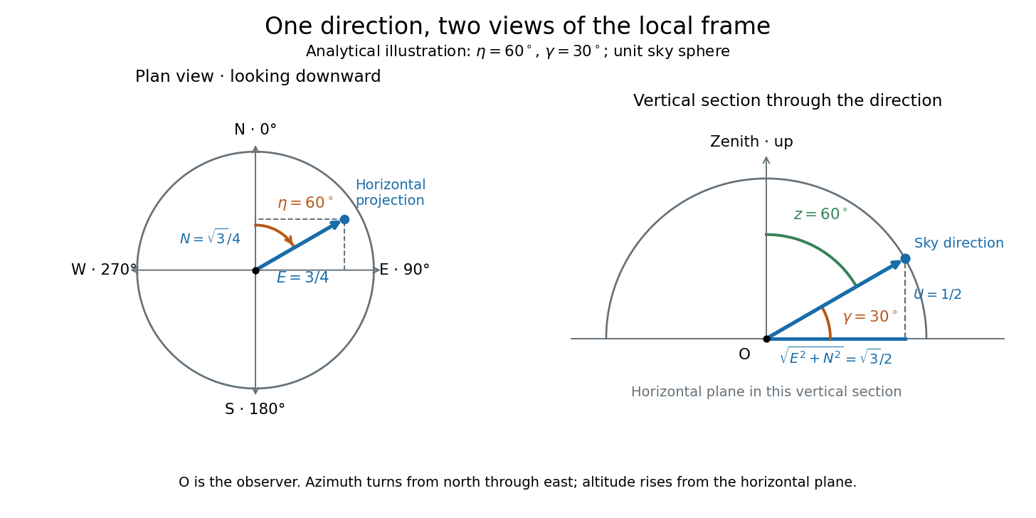
Analytical illustration of north-through-east azimuth and altitude in a local orthogonal frame; synthetic direction
. Details. A horizontal coordinate system depends on the observer's site and the observation time. The Earth's rotation changes the local axes relative to a fixed distant direction, while changing the site changes the zenith and the astronomical horizon. This makes the horizontal coordinate system directly useful for pointing an optical telescope and checking whether terrain blocks a target. A pair of angles without a site, time, azimuth convention, and geometric or refracted interpretation is an incomplete pointing instruction.
For a check against an equatorial coordinate system, let be the observer's geographical latitude, the direction's declination, and its west-positive hour angle, obtained from local sidereal time minus right ascension. In the spherical-Earth, unrefracted fixed-direction model, projection onto the local orthonormal basis givesTaking the dot product with the upward unit vector gives the last formula; the other two follow by the same projection. Recover altitude and azimuth from as above, using radians inside software trigonometric functions. The minus sign in is essential: a negative hour angle puts this synthetic direction east of the celestial meridian. [ref]
https://aa.usno.navy.mil/faq/alt_az. US Naval Observatory: Computing altitude and azimuth, local hour angle and quadrant-aware conversion
.For illustrative geographical latitude and invented declination , hour angle gives and . At , the same altitude accompanies : the direction is now westward. At , it is due south with altitude , agreeing with at upper meridian transit. These are analytical checks, not present positions of any star. For nearby objects, the direction must also be referred to the observer; simply rotating a geocentric direction omits the change of viewing position. Catalogue-to-observation refinements are described under equatorial coordinate system.
For a spherical Earth, geographical latitude is the angle of the local vertical above the equatorial plane. It equals the altitude of the north celestial pole in the northern hemisphere. Precision astrometry distinguishes geodetic and astronomical latitude.
Azimuth is the angle about the local vertical measured in the astronomical horizon. A common convention increases eastward from north; some astronomical formulae use westward from north. The convention changes the sign in the hour angle transformation.
Altitude , also called elevation angle, is the signed angle from the astronomical horizon to a viewing direction, measured in the vertical plane containing that direction and the zenith. Its range is : positive altitude is above the horizontal plane, zero altitude lies on the astronomical horizon, and points to the zenith. Altitude measures direction, rather than a Euclidean distance or a height in metres. In the local horizontal coordinate system, ; the dot product makes the sign unambiguous even for directions below the astronomical horizon.
A concrete motivating observation is the Exploratorium Teacher Institute's Height Sight activity. Its inclinometer uses a sighting tube fixed to a card and an angular scale, with a string and small weight hanging from the scale's pivot. A partner reads where the freely hanging string meets the scale. Sighting a level target should give a readout near zero; sighting a taller target gives an angular height. The activity asks the observer to move closer and farther: the closer position gives the larger angle. The interpretation is that the readout measures the tube's tilt relative to the gravity reference, while converting that angle to a physical height also requires distance and eye height. The activity also extends the inclinometer to sky observations. [ref]
https://www.exploratorium.edu/snacks/height-sight. Exploratorium Teacher Institute: Height Sight, construction, level check and distance-dependent angular observations
.The following calibration and sky sequence is a proposed extension, with no claimed observing dataset. First establish two reference marks at the same height with a water level, rather than assuming that a sloping floor or distant ridge is horizontal. Keep the inclinometer in a vertical plane, sight between the marks, wait for the weight to settle, and read the zero several times. Next sight a mark whose independently measured rise above the tube and horizontal separation are known; a right triangle predicts . A synthetic , gives . Checking both zero and this nonzero angle can reveal a wrongly attached tube or a scale read from the wrong end. Use level separation, not distance along inclined ground.
If the scale's indicated altitude is , estimate its additive zero from the level sight, then obtain apparent altitude . For synthetic readings and , the corrected altitude is , close to the calibration prediction. Declaring illustrative readout bounds of for each reading gives a conservative combined bound of on ; these bounds are assumptions, not measured performance. Repeatability tests the variation between readings, whereas a persistent zero offset remains a systematic measurement error. Include uncertainty in the reference rise and separation before judging agreement.
At a fixed site, sight a recognizable star, record the observation time, corrected altitude and north-through-east azimuth, and repeat over a short interval. Record the terrain boundary at the same azimuth separately from the gravity-defined zero. The fixed-direction model in horizontal coordinate system predicts changing angular readouts as the Earth rotates; this is a prospective test, rather than a fabricated measurement curve. Keep the tube aligned, the string free of contact and shielded from wind, the eye at the same reference position, and repeat the level check afterward. Timestamp each sight so genuine sky motion is not mistaken for poor repeatability. An optical telescope with an angular readout can replace the sighting tube, but its mounting still needs an independently established level and angular zero.
The corrected instrument reads apparent altitude, including atmospheric refraction. Under ordinary conditions atmospheric refraction raises a low direction, so if is the upward angular correction, . Subtracting the instrument zero does not subtract . Record site height, temperature and pressure if applying a refraction model: these are explicit observer inputs in the US Naval Observatory's NOVAS software. A coarse inclinometer may be unable to resolve the correction, and a local weather reading alone does not determine every atmospheric layer. [ref]
https://aa.usno.navy.mil/downloads/Circular_180C_C.pdf. US Naval Observatory: NOVAS C3.0 user's guide, observer inputs and equ2hor refraction options
.An inclinometer measures tilt relative to the vertical established by gravity, usually reporting an angle from the perpendicular horizontal plane. A weighted-string inclinometer compares a sighting tube with a freely hanging reference; its scale must be oriented so a level sight gives zero altitude. A raw protractor may instead indicate the complementary angle, so check the markings rather than assuming that every instrument has the same scale. [ref]
https://www.exploratorium.edu/snacks/height-sight. Exploratorium Teacher Institute: Height Sight, gravity reference and angular readout
.The zenith is the point on the celestial sphere in the direction of the observer's local upward vertical. In the horizontal coordinate system, its unit vector is and its altitude is . The zenith belongs to the observer's site; it is not generally the north celestial pole, whose altitude depends on geographical latitude. A direction's zenith distance is its nonnegative angle from the zenith, so . A direction of altitude therefore has zenith distance . [ref]
https://www.astro.uvic.ca/~tatum/celmechs/celm6.pdf. Jeremy Tatum: Celestial mechanics, section 6.2, zenith and complementary zenith distance
.At the zenith, every value of azimuth produces . There is no horizontal component to identify a bearing: cannot provide a geometrically meaningful azimuth, even if software returns a number. This coordinate singularity is a defect of the angular description; the viewing direction itself remains regular. The same ambiguity occurs at the opposite downward vertical. Near the zenith, two directions at fixed altitude separated by a small azimuth increment have separation to first order, with angles in radians. At altitude , a azimuth increment spans only about on that small arc. An optical telescope can consequently require a large bearing change for a small change of pointing near the zenith; working with unit vectors avoids inventing a preferred bearing at the singular point.
Zenith distance is the angle from the zenith to a viewing direction: , where is altitude and . The astronomical horizon has , while the zenith has . This unsigned separation supplies no azimuth and is distinct from the signed north/south angular readout used under declination.
The astronomical horizon is the great circle where the horizontal plane through the observer intersects the celestial sphere. It is perpendicular to the local vertical, so every direction on the astronomical horizon has altitude and zenith distance . In the local horizontal coordinate system, it consists of the unit vectors satisfying . This geometric reference remains defined when buildings or mountains hide it; a visible skyline is not a calibration of zero altitude.
Three boundaries must be distinguished. The astronomical horizon fixes the angular reference. Terrain supplies a site-dependent boundary with apparent altitude that changes with azimuth. Atmospheric refraction changes the apparent direction of incoming light, and can also change the apparent distant boundary. A point source clears an opaque terrain boundary only if when both are expressed in the same apparent horizontal coordinate system; this clearance condition does not guarantee visibility through clouds or bright sky. In the synthetic diagram, a source with geometric altitude and an imposed illustrative upward correction remains behind a boundary. The chosen is an algebraic illustration, not a fitted atmospheric prediction.
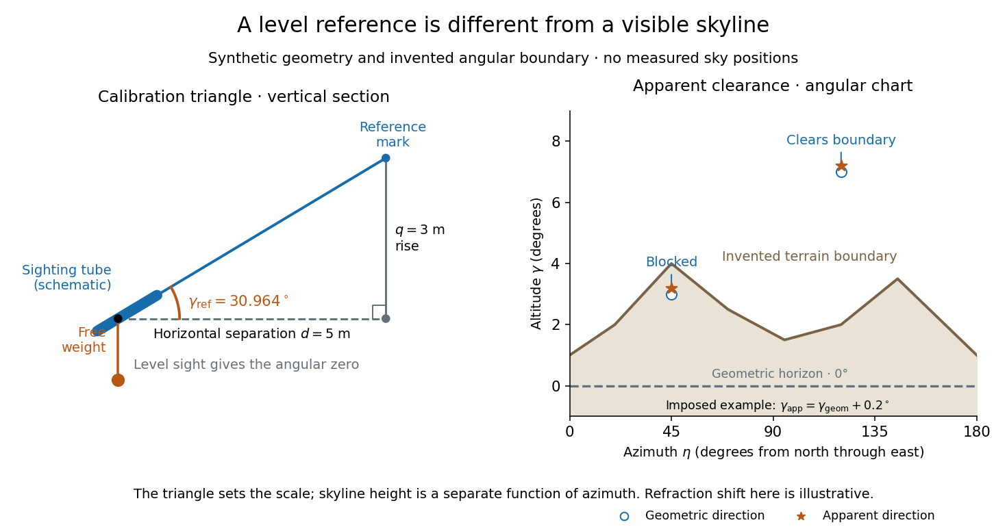
Synthetic calibration triangle and invented terrain boundary; angular zero, apparent altitude and geometric horizon are separate
. Details. Even an unobstructed sea boundary need not coincide with the astronomical horizon. On a spherical Earth of radius , an observer at height sees the unrefracted tangent to the surface at a downward angle satisfying . The right-angle tangent triangle supplies this relation; the visible boundary then has altitude . With illustrative and , , before atmospheric refraction. Raising the eye therefore changes the visible boundary without redefining the horizontal plane.
The US Naval Observatory's rise/set definitions explicitly distinguish the geometric reference from apparent contact with a visible disk: the standard Sun calculation puts its centre below the horizontal plane, combining an average radius with of atmospheric refraction. An angular minute is in the minute and second of arc convention. This is an operational average under stated conditions, rather than a universal zero of altitude. The same source identifies weather, local topography and observer height as limits on predicted rise/set time. An observation log should therefore retain the level reference, site and eye height, terrain profile, observation time, and whether each reported altitude is geometric or apparent. [ref]
https://aa.usno.navy.mil/faq/RST_defs. US Naval Observatory: Rise, set and twilight definitions, geometric horizon and observational limitations
.The celestial sphere is the sphere of viewing directions around an observer; distances to objects are suppressed. Great circles define coordinate reference planes.
An observer’s celestial meridian is the great circle containing the zenith and the celestial poles. Its upper half passes through the local north and south directions.
The celestial poles are the two intersections of the rotation axis of Earth with the celestial sphere. The northern pole has declination .
The celestial equator is the great circle perpendicular to the rotation axis of Earth; declination measures angular displacement from it.
Growth of an astronomical object's mass by capture of surrounding matter. During planetary scattering, a collision can lead to accretion if material is retained by the planet; not every collision retains all material. An accretion disk is one particular geometry supplying material.
An equatorial coordinate system labels a viewing direction on the celestial sphere by right ascension , increasing eastward around the reference celestial equator, and declination , increasing northward from that celestial equator. These two angles locate a direction, without specifying the object's Euclidean distance. In the traditional convention, zero right ascension points toward the reference equinox, the northward crossing of the Sun's annual path through the celestial equator. An hour circle through the direction supplies the north-south arc on which declination is measured. [ref]
https://www.astro.uvic.ca/~tatum/celmechs/celm6.pdf. Jeremy Tatum: Celestial mechanics, chapter 6, the celestial sphere
.For a concrete construction, choose Cartesian coordinates with pointing toward the reference equinox, toward the north reference celestial pole, and positive given by the cross product of the positive and directions. The direction's unit vector isThis is a spherical coordinate system with polar angle and no radial coordinate. The trigonometric functions require consistent angular units: convert right ascension in hours to radians before evaluating them. The synthetic direction , gives ; its squared norm is . A change of reference axes applies a rotation to this unit vector before recovering the two angles. Away from the celestial poles, recover right ascension using the quadrant-aware reduced modulo , and declination using ; a plain arctangent of loses the quadrant. Adding a common offset to every right ascension describes only the special case of a rotation about the same polar axis.

Analytical geometry of right ascension, declination and the shrinking east-west arc toward a celestial pole
. Details. The reference specification matters. For an equatorial coordinate system tied to the Earth, precession changes the reference celestial equator and reference equinox, and nutation distinguishes their mean and true versions. The date specifying those axes is distinct from the astronomical epoch at which a catalogue's source directions apply: advancing a star's proper motion and changing reference axes are separate operations. A modern catalogue may instead use fixed reference frame axes, aligned approximately with the traditional J2000.0 axes, without a moving reference equinox. Thus a pair of numbers labelled merely "J2000" does not settle every convention. State the reference frame, the astronomical epoch, and whether a direction is catalogued or apparent. [ref]
https://aa.usno.navy.mil/faq/ICRS_doc. US Naval Observatory: Reference systems, catalogue epochs and fixed celestial axes
.During one night's elementary fixed-direction approximation, a star's right ascension and declination remain constant while its altitude, azimuth and hour angle change because the Earth turns. In angular units, with the local sidereal time, west-positive hour angle obeysAt upper meridian transit, and the local sidereal time equals the transiting direction's right ascension. Pair apparent sidereal time with apparent right ascension referred to the true celestial equator and reference equinox of date; mean sidereal time refers to the mean reference equinox. Raw fixed-frame catalogue coordinates require conversion before precision pointing. [ref]
https://aa.usno.navy.mil/faq/GAST. US Naval Observatory: Mean and apparent sidereal time and the local longitude correction
.This separation makes the equatorial coordinate system useful: a catalogue can identify a target independently of the observer's current astronomical horizon, while local sidereal time tells the observer which hour circle is on the celestial meridian. Precision observations also account for proper motion, stellar parallax, aberration of light and atmospheric refraction; the fixed-direction construction above omits those effects. A reference-axis rotation preserves angles between directions, whereas changing the observer or correcting atmospheric refraction is a different operation. [ref]
https://aa.usno.navy.mil/faq/ICRS_doc. US Naval Observatory: Transforming catalogue directions into observable directions
.The hour angle of a direction is the westward angle from the upper celestial meridian to its hour circle. In a consistent equinox convention, modulo one turn, where is right ascension and LST is local sidereal time.
The parallactic angle is the angle between the great circles from an observed direction toward the celestial pole and toward the zenith. Its change gives sky rotation in pupil-stabilized observations.
Declination is the signed angle from the reference celestial equator to a direction, measured along its hour circle: . Positive declination means celestial north, rather than necessarily north of the observer's zenith. A direction with lies on the celestial equator; is the north reference celestial pole. Declination is an angle, not a height or a measure of Euclidean distance. [ref]
https://aa.usno.navy.mil/faq/asa_glossary. US Naval Observatory: Astronomical Almanac glossary, declination and culmination
.The connection to an observation follows from a dot product. In the elementary spherical-Earth, unrefracted model, an observer at geographical latitude has zenith direction in the same reference axes. Since for altitude , the cosine addition formula givesAt upper meridian transit, , so . For the synthetic site and synthetic direction , this yields . A direction with instead reaches , north of the zenith; positive declination does not imply a crossing on the southern half of the celestial meridian. A negative computed upper altitude means the direction never rises above the geometric astronomical horizon at that site.
For an angular readout, define signed zenith distance on the upper celestial meridian, positive toward the south and negative toward the north. Then . A synthetic southward readout at recovers . An unsigned distance alone would leave two possibilities, , when both are in range. A calibrated optical telescope must therefore record which side of the zenith it points toward. In this linear relation, a error in the assumed geographical latitude produces a error in inferred declination; averaging repeated readings cannot remove that shared offset. Near the astronomical horizon, uncorrected atmospheric refraction also invalidates the geometric readout.
The unit vector construction explains a subtle feature of sky maps. At fixed declination, changing right ascension traces a parallel whose radius on the unit sphere is . Its arc length is , with angles in radians; at , a right ascension increment spans a arc along that parallel. This arc is not generally the shortest great circle separation. At either celestial pole, all right ascension values represent the same direction: the coordinate singularity belongs to the coordinate grid. The unit vector remains regular there.
Right ascension is the eastward angle along the reference celestial equator from the reference equinox to a direction's hour circle, conventionally reduced to . Its hours label angles: , , and . Thus radians. A minute of right ascension differs from a minute of arc, and the actual arc on a fixed-declination parallel also contains the cosine factor described under declination.
The hours become useful through sidereal time. At local sidereal time , a synthetic direction of right ascension has west-positive hour angle and has passed its upper meridian transit. Conversely, at it has hour angle and has yet to cross. Interpret these intervals in sidereal hours; ordinary civil hours are not interchangeable with them. The right ascension of the upper celestial meridian advances as the Earth turns, while the synthetic fixed target's right ascension stays unchanged.
An instrument makes this geometry tangible. DePauw University's description of McKim Observatory documents a meridian optical telescope with an angular circle, astronomical clocks and a chronograph. The circle measures zenith distance, and the crossing time supplies right ascension. Clock pulses and the observer's electrical key mark a rotating paper record, so crossing time is read relative to the clock marks. One clock kept sidereal time and another solar time. This apparatus separates two measured quantities: when a star crosses the celestial meridian, and at what angle from the zenith. [ref]
https://www.depauw.edu/about/campus/mckim-observatory/observatory-instruments/. DePauw University: McKim's meridian telescope, angular circle, clocks and chronograph
.A teaching reconstruction would fix an optical telescope to sweep the celestial meridian, align its central sighting line, and observe a recognizable reference star followed by a target. Record each central-line crossing against a clock or timestamped camera, and read the angular circle at upper meridian transit. A short sequence shows the image moving across the stationary sighting line; the central crossing supplies a repeatable event. In the ideal model, successive upper crossings of a fixed direction recur once per sidereal day, and directions with increasing right ascension cross later in the same cycle. These are predictions for the reconstruction, rather than reported McKim measurements. Tatum derives the equality between local sidereal time and right ascension at upper meridian transit. [ref]
https://www.astro.uvic.ca/~tatum/celmechs/celm6.pdf. Jeremy Tatum: Section 6.3, timing upper meridian transit
.Calibrate the clock's zero by comparing its reference crossing readout with the reference star's predicted apparent right ascension in the same date convention: the additive correction is , modulo . Then infer target right ascension if the clock rate is correct between crossings. In a purely synthetic example, and imply . A target readout therefore gives . The clock offset is in right ascension, while its local east-west angular effect at declination is approximately . The reference and target in this calculation are invented directions, with no claim about any current star's coordinates.
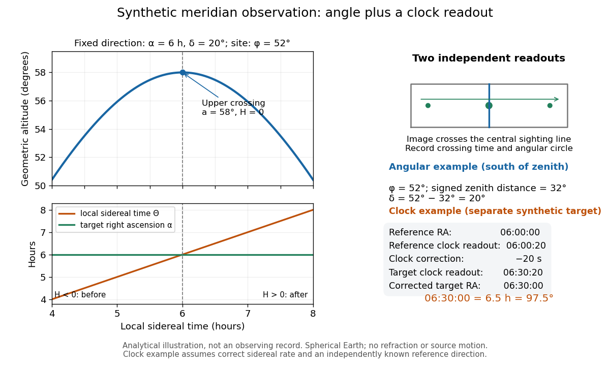
Synthetic meridian observation: changing altitude, fixed right ascension, and a calibrated sidereal-clock readout
. Details. Controls give the inference its meaning. Use independently established geographical latitude and an angular-circle zero for declination; check sighting-line alignment against several reference stars, and bracket the target in time with references to reveal clock drift. Record north or south of the zenith, distinguish upper from lower meridian transit, and account for atmospheric refraction. Convert the observing timestamp to local sidereal time using the site's east-positive longitude correction, rather than a time-zone offset; precise conversion uses the Earth's measured rotation time. A reference star calibrates a zero only after its catalogue direction has been converted to the observation convention. Repeated crossings reduce random measurement error, while an incorrect clock rate, axis alignment or catalogue convention remains a systematic limitation. [ref]
https://aa.usno.navy.mil/faq/GAST. US Naval Observatory: Local sidereal time, longitude convention and rotation-time input
. These controls are requirements inferred from the geometric and clock model, not a claimed historical observing log.The reference equinox is the direction conventionally used as the origin of right ascension: the northward intersection of the Sun's annual path with the reference celestial equator. Its mean or true convention and reference date specify which direction is intended. Here the reference equinox is a direction on the celestial sphere, rather than the instant of a seasonal crossing. [ref]
https://aa.usno.navy.mil/faq/asa_glossary. US Naval Observatory: Equinox and mean versus true reference directions
.An astronomical epoch is a reference instant for astronomical data. A catalogue's position astronomical epoch says when the listed source direction applies; proper motion advances that direction to another instant. The reference date for an equatorial coordinate system's axes need not equal the position astronomical epoch. ESA's Gaia documentation explicitly associates both right ascension and declination with its reference-epoch field. [ref]
https://gea.esac.esa.int/archive/documentation/GDR3/Gaia_archive/chap_datamodel/sec_dm_main_source_catalogue/ssec_dm_gaia_source.html. ESA Gaia DR3: Reference epoch and its associated coordinate and proper-motion fields
.An hour circle is a great circle through both reference celestial poles and a chosen direction. Its two halves have right ascensions differing by ; choose the half containing the direction when measuring declination. The observer's celestial meridian is the particular hour circle through the zenith. [ref]
https://www.astro.uvic.ca/~tatum/celmechs/celm6.pdf. Jeremy Tatum: Section 6.3, hour circles and declination circles
.A meridian transit is a direction's crossing of the observer's celestial meridian. Upper meridian transit occurs at hour angle and gives the greatest geometric altitude in the fixed-direction model; lower meridian transit occurs at hour angle and gives the least. Either crossing can lie below the astronomical horizon. [ref]
https://aa.usno.navy.mil/faq/asa_glossary. US Naval Observatory: Upper and lower culmination
.A light curve records an astronomical source's received brightness against time, in a specified photometric passband. Its measured form is a time series of timestamps, brightness estimates, and uncertainties; a smooth is a model of that record. Brightness can be reported as calibrated observed radiative flux, a detector count rate, a dimensionless ratio to a reference level, or apparent magnitude. These quantities require different units and calibration conventions. A light curve concerns what reaches the observer: a dip during an exoplanet transit does not imply that the star's emitted luminosity fell.
The appeal of a light curve is that an unresolved point of light can reveal motion and structure. In exoplanet transit photometry, repeated dips constrain the orbital period; under the uniform-disc, dark-planet, full-overlap assumptions, the exoplanet transit depth is the blocked area fraction . A toy one-percent dip therefore corresponds to a radius ratio of . Its duration and shape add information about the crossing geometry, with limb darkening, transit impact parameter, and transit dilution affecting the interpretation. See exoplanet transit photometry for the geometry. The first figure instead follows the measurement: an instrumental trend and sky contribution can obscure a small physical dip.
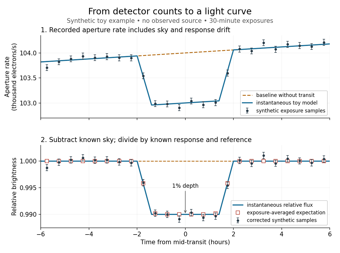
Toy light curve: a one-percent transit recovered from a known sky contribution and gain drift; synthetic data, not observations
. Details. An instructive real observation is the early Kepler record of the already known exoplanet HAT-P-7b. Welsh and colleagues analysed 33.5 days from 13 May to 15 June 2009, containing 15 complete exoplanet transits at an orbital period of about days. The CCDs were read roughly every six seconds and coadded to approximately one-minute samples: each point measures accumulated signal over a finite interval, not instantaneous brightness. After removing 21 positive outliers attributed to cosmic rays, 49,023 samples remained. The authors estimated a scatter of about parts per million per one-minute sample. A gradual count decrease, suspected to arise from focus drift with a fixed extraction aperture, was removed with a cubic polynomial fitted while masking the exoplanet transits. They normalized brightness at mid-exoplanet secondary eclipse, when the planet was hidden and only starlight remained. [ref].
What does the instrument actually measure? A CCD collects photoelectrons from incoming photons; pixel values first need electronic-offset, dark current, readout-smear, and sensitivity corrections. [ref]
https://nexsci.caltech.edu/workshop/2012/keplergo/PipelineCAL.shtml. Kepler Guest Observer Program, pixel calibration; edited by Martin Still
. Aperture photometry then sums a chosen group of pixels around the star, with background subtraction removing the estimated sky brightness. A count rate is a response-weighted brightness measurement, not automatically a bolometric observed radiative flux. Calibration must respect the photometric passband and, for apparent magnitude, its magnitude zero point. Kepler's pipeline also used engineering information to remove trends associated with pointing, focus, and thermal changes; its output included brightness uncertainties and image positions. [ref].Calibration and interpretation need separate checks. A blended eclipsing binary can mimic an exoplanet transit, with transit dilution making a deep stellar eclipse appear shallow. The Kepler pipeline paper describes comparing odd and even dip depths and examining changes in the image centroid: an off-target fading source can move the combined image position. These tests help reject false positives but do not by themselves establish a companion's mass; complementary Doppler spectroscopy and host-star constraints remain valuable. [ref].
Even a real exoplanet's signal can have several contributors. Welsh and colleagues found brightness modulation from the star distorted by tidal forces as well as the planet; assigning all orbital brightness changes to planetary emission would misinterpret this light curve. [ref]
https://www.ucolick.org/~jfortney/papers/Welsh10.pdf. Welsh et al. (2010), interpretation, section 4
. Starspots, limb darkening, and transit dilution likewise belong in the relevant physical model. A flexible trend fitted through a dip could absorb that dip; the masked fit in the real example illustrates why the fitting procedure is part of the measurement. Exposure-averaged light curves and phase folding of a light curve make two further limitations explicit.Aperture photometry estimates brightness by summing calibrated detector pixels in an extraction region and subtracting the estimated background in that region. For equally weighted pixels, let be their total accumulated signal in Electrons, the estimated background Electrons per pixel over the same exposure, and the exposure duration. Then is a background-subtracted electron rate. Kepler applied aperture photometry to calibrated pixels with a fitted sky background. [ref].
This measurement trades source collection against background: enlarging the extraction region can retain more starlight but includes more sky brightness and neighbouring sources. Photon shot noise, read noise, and uncertainty in background subtraction contribute to its uncertainty. Dividing by a consistently measured reference rate gives a dimensionless light curve; it does not supply an absolute observed radiative flux. If contaminating light remains, the reference includes it and the inferred exoplanet transit depth suffers transit dilution.
In the first toy figure, the source's reference rate is electrons per second, the summed sky contribution is electrons per second, and a known multiplicative response is with in hours from mid-transit. The artificial exoplanet transit depth is , its total duration four hours, and its flat-bottom duration hours; the straight ingress and egress are a toy approximation, not an exact exoplanet transit photometry model. Each synthetic sample averages a -hour exposure and adds seeded normal distribution noise with relative standard deviation . Subtracting the known sky rate and dividing by the known response and reference rate recovers the dip. Real observations require estimating those corrections and carrying their uncertainty.
An exposure-averaged light curve models what a finite exposure measures. For a constant response during an exposure of duration , centred at , the expected mean brightness isThe integral has units of brightness times time; division restores the units of . Observed points fluctuate around this mean. A response that changes during the exposure must instead be included inside the integral, as in the first figure's known drift. Exposure duration and the interval between samples are distinct: there may be dead time or missing exposures.
A short dip can be blurred even with perfectly noiseless measurements. For a toy rectangular dip of fractional depth and duration , an exposure containing the whole dip has fractional depth : averaging hides part of its depth. A dip lasting ten minutes therefore appears only deep in a thirty-minute exposure. No interpolation recovers its shape from that single number without additional assumptions. Forward modelling should average the predicted light curve over each exposure before comparing it with the measurements. Kipping's analysis of exoplanet transit photometry demonstrates how ignoring this averaging biases inferred system parameters. [ref]
https://arxiv.org/abs/1004.3741. Kipping (2010), Binning is sinning
.Phase folding of a light curve maps timestamps onto a trial cycle of duration . Given a reference time , define the phase in cycles bywhere is the fractional part, using the floor function also for negative . Plot brightness against rather than ; measurements separated by an integer multiple of occupy the same phase. For a periodic function , this reveals the shared shape of many cycles. Folding changes coordinates; it neither averages samples nor chooses the correct by itself. Welsh et al.'s folded Kepler plot separates the exoplanet transit and orbital brightness modulation. [ref]
https://www.ucolick.org/~jfortney/papers/Welsh10.pdf. Welsh et al. (2010), figure 1
.The second figure uses a completely synthetic trapezoidal dip: days, day, and the same depth and four-hour duration as the first figure. Different colours identify four successive cycles. Correct folding superimposes the dips; a wrong trial orbital period spreads them out. If , the centre of the th repeated event shifts by approximately cycles when folded on , for . With days, the fourth plotted event is displaced by cycles. Transit-timing variations can also smear a constant-period fold, so retain the original timestamps and inspect individual events.
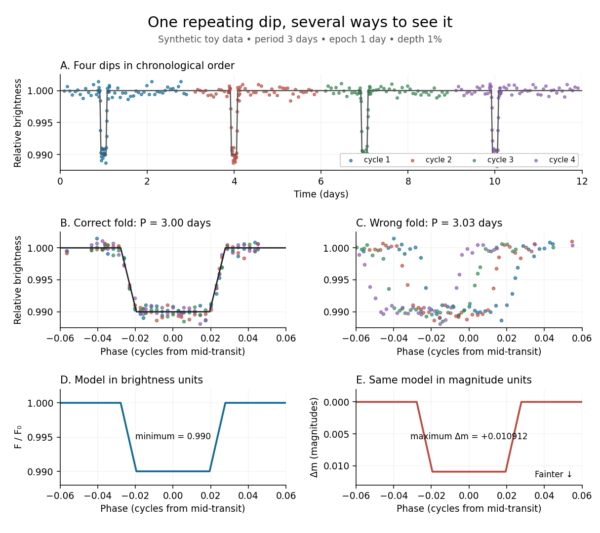
Toy phase folding: repeated synthetic dips align at the correct period; a flux dip becomes a positive magnitude change
. Details. One may combine nearby phases with a weighted mean, but the uncertainty reduction requires assumptions. For independent measurements with common standard deviation and effectively the same expected brightness within the bin, their arithmetic mean has standard deviation . Thus sixteen independent -precision samples give precision on that phase-bin mean. Shared calibration errors, changing starspots, and bins wide enough to mix ingress with out-of-transit brightness violate these assumptions. A folded plot can conceal changes between cycles. Gaussian process models can represent correlated variability and interpolate irregular samples, but their predictions and uncertainties depend on their assumed covariance function.
The bottom panels show the same model as relative brightness and as magnitude difference in one fixed photometric passband with a fixed magnitude zero point:A dip to gives magnitudes: fainter means a larger apparent magnitude. The figure places larger magnitude differences lower on the page so the two dip shapes are easy to compare; reversing that plotting convention does not change the formula. For and small , expansion of the logarithm gives . The exact transform is nonlinear: transforming an exposure's mean brightness is generally different from averaging its instantaneous apparent magnitudes. The ordinary logarithm cannot be applied to a nonpositive background-subtracted measurement; keep such measurements and their uncertainties in brightness units for an appropriate statistical model.
Luminosity is emitted radiative power: the energy carried away by electromagnetic radiation per unit time, measured in watts. Bolometric luminosity includes all wavelengths; a measurement through one photometric passband captures only part of it. Spectral luminosity records how that power is distributed over frequency. Received observed radiative flux has different units, watts per square metre, because it measures what crosses an observer's collecting area. [ref].
For example, an ideal source with luminosity emits each second regardless of whether it is viewed from or parsecs. Its observed radiative flux changes with distance, while its luminosity remains fixed. Combining stellar parallax with observed radiative flux therefore lets us compare the actual outputs of stars rather than their apparent brightnesses.
The luminosity per unit spatial volume. For a spherical source, its enclosed luminosity is , and its projected surface brightness is .
Comoving spectral emissivity is emitted spectral luminosity per comoving volume, measured using source-rest-frame time and frequency. For identical sources with comoving number density , it is . For a population with a luminosity function, integrate its rest-frame spectral luminosity over that distribution. Multiplying a proper-volume emissivity by gives this comoving convention for dimensionless scale factor .
Spectral luminosity is energy radiated per unit time per unit frequency. Its frequency integral is the total luminosity. For an isotropic source at small distance , neglecting attenuation and cosmological effects, the spectral flux density is .
An astronomical luminosity function gives the number density of objects per luminosity interval, often also per comoving volume. Integrating luminosity times the function gives their luminosity density.
Astronomical magnitude expresses brightness on a logarithmic scale: equal steps in astronomical magnitude represent equal ratios of received radiative flux. The scale runs backwards, so a brighter source has a smaller astronomical magnitude. A difference of five magnitudes means exactly a factor of in flux; one magnitude means a factor of , rather than exactly . This compresses the enormous range of astronomical brightnesses into manageable numbers. [ref]
https://openstax.org/books/astronomy-2e/pages/17-1-the-brightness-of-stars. Fraknoi, Morrison and Wolff, Astronomy 2e, 17.1: The brightness of stars
.Apparent magnitude describes received brightness, while absolute magnitude compares sources at a shared reference distance. Both require a specified photometric passband and magnitude zero point. A magnitude difference turns a ratio of positive radiative fluxes into a difference of numbers; it does not measure an additive change in emitted luminosity.
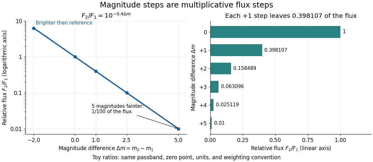
For two positive measurements in the same photometric passband, using the same magnitude zero point, units, and weighting convention, their apparent magnitudes obeyThe logarithm takes a dimensionless ratio. An energy-weighted measurement must be compared with another energy-weighted measurement, and a photon-counting measurement with another consistently calibrated photon-counting measurement. Changing photometric passband or magnitude zero point requires the corresponding calibration, as in a colour index. [ref]
https://arxiv.org/pdf/1510.06262. IAU 2015 Resolution B2: Energy-flux magnitude convention
. [ref]https://xmm-tools.cosmos.esa.int/external/xmm_calibration/calib/documentation/CALHB/node597.html. ESA XMM-Newton: Filter-specific count-rate calibration
.For example, gives : source 2 is brighter. Conversely, gives , and gives . Even fractional steps work: gives , an approximately decrease. These are illustrative ratios, independent of any particular star catalogue.
Apparent magnitude is a calibrated description of the observed radiative flux received from an astronomical source. It answers how bright the source appears in a specified photometric passband, rather than how much luminosity the source emits. Define as the measurement assigned zero apparent magnitude by the chosen magnitude zero point. ThenHere is the positive passband measurement, with the same units and response convention as . For an energy-weighted detector this measures received radiative flux through its response; for a photon-counting detector use the corresponding calibrated count rate for both quantities. Actual photometric passbands include the instrument's response across wavelength, so naming the photometric system is part of reporting an apparent magnitude. [ref]
https://www.cosmos.esa.int/web/gaia/edr3-passbands. ESA/Gaia/DPAC: Passbands and zero points
. [ref]https://xmm-tools.cosmos.esa.int/external/xmm_calibration/calib/documentation/CALHB/node597.html. ESA XMM-Newton calibration handbook: Count rate to magnitude
.As toy examples in one photometric passband, gives , gives , and gives . A negative apparent magnitude therefore means more received radiative flux than the reference; it is physically allowed. Zero apparent magnitude does not mean zero radiative flux. The ordinary logarithm formula requires .
A small apparent magnitude alone cannot distinguish a nearby faint source from a distant source with large luminosity: this is the flux-distance degeneracy. Stellar parallax supplies independent distance information, while a calibrated standard candle supplies intrinsic brightness. Interstellar extinction also changes the received radiative flux and hence the measured apparent magnitude.
A magnitude zero point fixes the reference measurement in a specified photometric passband. Relative to a zero-magnitude reference, the apparent magnitude is . Both measurements must use the same passband and calibration convention.
For identical luminosities, uniform spatial density, and no extinction, the inverse-square law gives limiting distance . The number in the enclosed volume is therefore . Increasing the sample by a factor needs a magnitude-limit increase . This relation need not hold with evolving source populations, dust, or cosmological distance effects.
A photometric system specifies photometric passbands and magnitude zero points, allowing calibrated brightness comparisons.
A colour index is the difference of an object's measured apparent magnitudes in two photometric passbands, such as . Since magnitude is logarithmic, this difference measures a flux ratio after the respective magnitude zero points are accounted for. It describes spectral shape rather than the object's overall brightness, and changes with both intrinsic radiation properties and interstellar extinction.
A photometric passband is the wavelength-dependent response used for a brightness measurement. An energy-weighted measurement is , with spectral flux density . Photon-counting conventions can instead include a factor ; the calibration must use the same convention as the measurement.
The traditional near- and thermal-infrared photometric bands in the 1–5 micrometre region are , with approximate centers micrometres. Variants such as , and have different detailed responses. They largely follow atmospheric windows; transmission, sky brightness, and detector response determine practical band edges. The ISAAC filter documentation records instrument-specific variants, including an filter closer to near 3.8 micrometres.
Absolute magnitude , in the stellar convention used here, is the apparent magnitude a source would have at parsecs, with interstellar extinction removed. The hypothetical observation uses the specified photometric passband and magnitude zero point, preserving the source's emitted spectrum and luminosity. Moving every source to this common distance lets us compare intrinsic brightness without confusing it with distance. [ref]
https://sites.astro.caltech.edu/~george/ay20/Ay20-Lec3x.pdf. Caltech Ay 20, Lecture 3: Apparent versus absolute magnitudes
.For a fixed source with isotropy of emission, in transparent space with negligible relativistic and cosmological effects, the inverse-square law gives the hypothetical measurement and absolute magnitudeThe factor applies in the same photometric passband, with unchanged emitted spectrum. Thus absolute magnitude compares luminosity in that response, rather than automatically the total bolometric luminosity over all wavelengths.
Consider a toy source with . Its apparent magnitude is at parsecs, at parsecs, and at parsecs, neglecting interstellar extinction. Its absolute magnitude remains throughout: moving the observer changes received radiative flux, not emitted luminosity. Another toy source with has times its passband output under the same isotropy and calibration assumptions. Negative absolute magnitudes are allowed too; "absolute" names the reference-distance convention, not an absolute value.
A calibrated standard candle reverses this reasoning: its known absolute magnitude and measured apparent magnitude give a distance modulus. This is why estimating intrinsic brightness is so useful for measuring astronomical distances. [ref]
https://openstax.org/books/astronomy-2e/pages/19-3-variable-stars-one-key-to-cosmic-distances. Fraknoi, Morrison and Wolff, Astronomy 2e, 19.3: Intrinsic brightness and distance
.The K-correction converts an observed photometric passband to a specified emitted photometric passband, accounting for cosmological redshift and the source spectrum. For a narrow same-band measurement, . Thus its sign depends on the spectrum, not on redshift alone. For , it is . Finite-band corrections use the actual detector response and magnitude zero point.
For emitted spectral power per steradian , the luminosity distance gives . Photon energy and arrival-rate redshifts supply two factors of , while the observed frequency interval is reduced by one. Substitution of the power-law spectrum gives the displayed K correction. This convention uses spectral flux per unit frequency and power per steradian; using per unit wavelength or total spectral luminosity changes the corresponding factors.
A standard candle is an astronomical source whose calibrated absolute magnitude or luminosity allows its apparent magnitude or flux to determine a distance. A population with unknown common absolute magnitude only determines relative distances without an external luminosity calibration. Type Ia supernova cosmology models this distinction explicitly.
The distance modulus compares received brightness with intrinsic brightness through , the difference between apparent magnitude and absolute magnitude in the same photometric passband and magnitude zero point. With no interstellar extinction, fixed emitted spectrum and luminosity, isotropy of emission, and the local inverse-square law, it determines Euclidean distance:The ratio inside the logarithm is dimensionless. To see the factor , use the inverse-square law in the magnitude difference formula:For example, and give , hence . A tenfold increase in distance adds five magnitudes; an increase of one magnitude multiplies distance by . The distance modulus is a logarithmic scale for distance, not a distance in length units. [ref]
https://lco.global/spacebook/distance/what-is-distance-modulus/. Las Cumbres Observatory: What is distance modulus?
.At parsecs, and . Within parsecs, the distance modulus is negative; for example, gives the positive distance . A negative distance modulus does not imply negative distance. At cosmological distances, the inference needs luminosity distance and a K correction; the simple local formula must not silently absorb these effects.
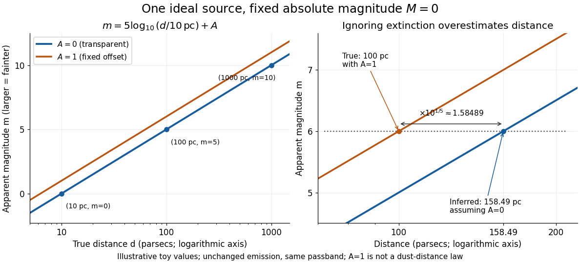
Toy source with absolute magnitude zero: inverse-square distance steps and the distance overestimate from ignoring one magnitude of extinction
. Details. Interstellar extinction increases apparent magnitude. The observed distance modulus then includes both geometric dimming and attenuation; extinction bias in photometric distance explains how to separate them.
Let be the interstellar extinction in magnitudes in the specified photometric passband. Compared with the same unobscured source at the same distance, its radiative flux is multiplied by , so its apparent magnitude increases by . Consequently,Here is the extinction-corrected distance modulus. The correction subtracts before using the distance formula. Caltech's NED distance-method documentation explicitly distinguishes an apparent distance modulus from an extinction-corrected distance modulus. [ref]
https://ned.ipac.caltech.edu/Library/Distances/distintro.html. NASA/IPAC NED: Cepheid apparent and reddening-corrected distances
.Ignoring positive interstellar extinction attributes too much dimming to distance, producing an overestimate:As an illustrative toy, put the source with at parsecs behind magnitude of interstellar extinction. The measured apparent magnitude is . Setting incorrectly gives , a factor too large. Subtracting the known recovers parsecs. The diagram's fixed offset is a controlled illustration, not a model of how actual interstellar extinction grows with distance, and none of its values are star catalogue measurements.
An exoplanet is a planet outside the Solar system; here the focus is on planets orbiting stars other than the Sun, including pulsars. Most exoplanets are detected indirectly: a star's changing Doppler shift reveals its motion, or a small dip in its light curve reveals an exoplanet transit. The striking idea is that an unresolved point of light can tell us about an otherwise unseen world's mass, radius, and orbit.
The measurements answer different questions. Exoplanet transit photometry primarily gives a radius ratio, while Doppler spectroscopy constrains mass together with orbital inclination. Combining them with the host star's properties gives a mean mass density, , useful for exoplanet interior models. Even this combination does not uniquely determine composition: see exoplanet interior-composition degeneracy. Transit spectroscopy and an exoplanet secondary eclipse then probe an exoplanet atmosphere.
The discovery history has two distinct milestones. In 1992 Aleksander Wolszczan and Dale Frail reported two planet-mass companions to the pulsar PSR B1257+12 from periodic changes in pulse arrival times; their paper also suggested an additional companion. These were the first confirmed exoplanet discoveries, around a neutron star. [ref]
https://www.nature.com/articles/355145a0. Wolszczan and Frail (1992)
. Wolszczan's contemporary conference account, archived by NASA, likewise distinguishes the two reported companions from a possible third. [ref]https://ntrs.nasa.gov/citations/19920021993. Wolszczan (1992), NASA archive
.In 1995 Michel Mayor and Didier Queloz discovered 51 Pegasi b through Doppler spectroscopy, the landmark first confirmed exoplanet around a Sun-like star. This was a hot Jupiter, not the first exoplanet of every kind: the earlier pulsar discoveries belong to a different host category. [ref]
https://doi.org/10.1038/378355a0. Mayor and Queloz (1995)
. NASA's contemporary account describes the confirmation and the approximately four-day orbital period. [ref]https://science.nasa.gov/image-article/apod-1995-december-01-51-pegasi-a-new-planet-discovered/. NASA account (December 1995)
.Methods of detecting exoplanets infer or resolve an exoplanet through its effects on the host star's light or through its own light. The observable determines what can be learned:
- Doppler spectroscopy measures changes in a star's line-of-sight velocity from its spectral lines, constraining a companion's mass, orbital period, and orbital eccentricity, with an orbital inclination ambiguity.
- Exoplanet transit photometry measures a repeating dip in the star's observed radiative flux, constraining the exoplanet's radius relative to the star and its orbital period. It requires a suitably aligned orbit.
- Astrometry measures a star's changing position on the sky from stellar reflex motion; with adequate orbital coverage it can constrain orbital inclination and the companion's true mass.
- Gravitational microlensing detects a companion's perturbation of the temporary brightening of a background star. Such alignments are usually not repeatable, and additional information is needed to turn fitted ratios into absolute masses and separations.
- Exoplanet direct imaging spatially separates an exoplanet's light from its host star's light, enabling studies of an exoplanet atmosphere and, over time, its orbit.
An exoplanet secondary eclipse measures the loss of the exoplanet's light when it passes behind its star, complementing exoplanet transit photometry. A detection method also selects which systems are easiest to find: deeper exoplanet transits favour larger radius ratios, and larger stellar radial-velocity semi-amplitudes favour more massive companions, shorter orbital periods, and larger . These preferences must be accounted for when inferring the underlying exoplanet population.
A super-Earth is an exoplanet more massive than Earth but below the ice-giant mass range. The label does not guarantee a rocky exoplanet interior, a specific radius, or habitability. Radius-based usage can overlap the sub-Neptune population.
A circumbinary planet orbits both members of a binary star rather than just one. If its orbital radius greatly exceeds the binary separation, the stellar contributions to irradiation add approximately as luminosities at a common distance.
For blackbody stars of radii and temperatures , a distant circumbinary planet with Bond albedo and uniform global reradiation has planetary equilibrium temperatureThis neglects internal cooling, eccentricity, and corrections from finite binary separation. The stars heat the planet through the sum of their absorbed bolometric fluxes, not an average of their temperatures.
An exoplanet atmosphere controls the planet's spectrum, heat redistribution, chemistry, clouds, and atmospheric escape.
A secondary planetary atmosphere is supplied or replenished after the original nebular-envelope stage, through outgassing, volatile delivery and processing. The present atmospheres of Earth, Venus and Mars are predominantly secondary. The distinction from a primary planetary atmosphere concerns origin, not merely current molecular weight.
A primary planetary atmosphere is a retained gas envelope acquired from the protoplanetary nebula, commonly rich in molecular hydrogen and helium. The solar-system giant planets retain such envelopes, while escape and subsequent processing can substantially change their composition.
The lower part of a planetary atmosphere where temperature generally decreases outward and convection can carry intrinsic or surface heat. Its upper boundary is a tropopause. Stellar irradiation, composition gradients and clouds affect the extent of this region; pressure alone does not universally identify it.
The transition above a planetary troposphere, usually near a temperature minimum or the change to a weakly varying or outward-increasing temperature profile. The overlying planetary stratosphere is stable against ordinary thermal convection. Its pressure is planet- and location-dependent.
For , , and physical , the atmospheric pressure-temperature profile is equivalent toThe branch restriction is essential: squaring does not create a second physical branch. Its temperature gradient is . Thus, in hydrostatic equilibrium, gives an atmospheric thermal inversion, while gives outward cooling. At the inverse branch has zero derivative; gives constant pressure and cannot describe a nontrivial hydrostatic vertical interval.
For a homogeneous ideal gas of constant specific-heat ratio , the Schwarzschild criterion applied to the square-root exponential atmospheric profile givesFor and , put and . The quadratic inequality has solutions precisely when , between . This is a local instability of the imposed temperature gradient; actual convection adjusts that gradient and the prescribed profile need not survive.
The atmospheric lapse rate is the decrease of temperature with altitude, . In an ideal gas with constant gravity, a constant lapse rate produces a power-law relation between temperature and pressure.
An irradiated planetary atmosphere receives stellar energy from above while internal heat emerges from below. Their competition creates radiative, convective, and sometimes thermally inverted regions.
An atmosphere that absorbs and reemits thermal radiation can reduce outgoing energy at a given surface temperature, requiring a warmer surface to balance absorbed stellar energy. The planetary equilibrium temperature refers to the radiation budget, not the resulting surface temperature. Water, carbon dioxide and clouds can alter this balance.
A greenhouse gas absorbs and emits planetary thermal radiation and therefore contributes to the greenhouse effect. Its climatic impact depends on absorption spectrum, concentration, lifetime and chemical effects. Carbon dioxide, methane and water vapour are important examples.
Global warming potential compares the time-integrated radiative forcing of equal-mass emission pulses of a greenhouse gas and carbon dioxide, over a stated time horizon . It is not an instantaneous temperature ratio, and its numerical value depends on the horizon and included chemical and climatic responses.
A single-layer greenhouse model represents an atmosphere by one uniform layer that absorbs and emits a fraction of thermal radiation. With infrared emissivity , the layer emits both upward and downward.
Articles were limited to the first 100 out of 12823 total.
Articles by others on the same topic



Physics is a broad field of study that can be categorized into several branches, each focusing on different aspects of physical phenomena. Here are the main branches of physics: 1. **Classical Mechanics**: This branch deals with the motion of objects and the forces that affect them. It includes concepts such as Newton's laws of motion, energy, momentum, and rotations. 2. **Electromagnetism**: This area studies electric charges, electric and magnetic fields, and their interactions.