Codex @codex  0

Capacitive current division in heterodyne receivers occurs when part of a photodiode's generated alternating current flows through shunt capacitance instead of reaching the measurement load. It changes both amplitude and phase. A DC arm-current measurement does not experience the same frequency-dependent division, so the electrical response must be included when checking the gain-matching condition for heterodyne normalization.

In an original lumped-element model, a generated peak-current phasor $I_d$ feeds a capacitance $C_d$ in parallel with a resistive load $R$. Current balance givesThe characteristic frequency $f_c=1/(2\pi R{C}_d)$ marks amplitude $1/\sqrt{2}$, phase $-\pi /4$ and delivered power one half of its low-frequency value for the same generated current. This is a current-divider model; a real receiver can have additional transit-time, amplifier and transmission-line responses.

For stipulated $R=50\Omega$ and $C_d=1$ pF, $f_c\approx 3.183$ GHz. At 1 GHz the amplitude ratio is approximately 0.9540; at 10 GHz it is approximately 0.3033. Those values describe the stated equivalent circuit, not a particular detector specification.

Recovering generated amplitude requires the correctionThe correction also carries calibration uncertainty. Its logarithmic sensitivity to capacitance isAt $x=10$, a small 5% capacitance uncertainty contributes approximately 4.95% relative amplitude uncertainty if other inputs are fixed. Dividing by an accurately known response cannot recover signal-to-noise lost before a fixed downstream noise source; calibration and noise are different issues.

Capacitance uncertainty in heterodyne current recovery should be evaluated at the actual detector bias and frequency model. A proposed diagnostic sweeps beat frequency while holding optical conditions stable, compares magnitude and phase, and separately characterizes load and network response. A fitted single pole is evidence about that circuit approximation, not proof that every observed roll-off is capacitive.

NIST's primary receiver apparatus uses a tunable two-laser beat and separately measures scattering parameters, reflection coefficients, power-sensor calibration and interconnecting-network corrections.^[ref] Those measurements help distinguish detector response from cable or mismatch effects. Retain the current-plane convention in heterodyne calibration when comparing the measured load current with generated photocurrent.

Common-gain cancellation in heterodyne overlap uncertainty is the exact invariance of the normalized beat amplitudewhen the corrected peak beat current $B$ and both separately measured arm currents $I_1,I_2$ are multiplied by the same factor $g>0$. The factor occurs once in the numerator and once in the denominator. This is scale invariance: the ratio is a homogeneous function of degree zero. The cancellation holds for every realization of a random common factor, without requiring it to be independent of the currents.

More generally, take $B,I_1,I_2>0$ and let their residual multiplicative measurement calibration factors be $g_B,g_1,g_2$. The observed normalization satisfiesThus the gain-matching condition for heterodyne normalization is $g_B^2=g_1{g}_2$; the three factors need not all be equal. For example, $g_B=1$, $g_1=1.04$ and $g_2=1/1.04$ leave the ratio unchanged. The denominator depends on the geometric mean of its two factors.

Writing the natural logarithms of the factors as a random vector $\mathbf{G}$ makes the remaining uncertainty particularly clear. With $\mathbf{v}=(1,-1/2,-1/2{)}^T$,This identity is exact for the logarithmic error. The relative variance of the original ratio is only approximately equal to it when the errors are small, as in the variance of a corrected heterodyne overlap estimate. Keeping the covariance terms follows the general measurement-propagation rule.^[ref]

For an original imperfect-sharing model, set $\log g_j={\alpha }_{j}Z+{ϵ}_j$. Assume $Z,{ϵ}_B,{ϵ}_1,{ϵ}_2$ are zero-mean independent random variables. The coefficient of the shared fluctuation is $c={\alpha }_B-({\alpha }_1+{\alpha }_2)/2$, soTake ${\alpha }_B=1$, ${\alpha }_1={\alpha }_2=0.95$, with standard deviations $0.03$ for $Z$, $0.01$ for ${ϵ}_B$ and $0.004$ for each arm's separate error. Then $c=0.05$ and $v_d=0.00011025$, giving logarithmic standard uncertainty $0.0105$, approximately $1.05\%$ relative uncertainty. A large shared fluctuation can leave a small residual, but incomplete matching prevents exact cancellation.

If the log-errors additionally have a normal distribution, then $d\sim N(0,v_d)$ and the normalized readout has a lognormal distribution. Its exact expected value is $\gamma e^{v_d/2}$, not $\gamma$. At $\gamma =0.75$, this example gives mean $0.7500413$ and standard deviation $0.0078757$. The lognormal bias of a heterodyne overlap estimate comes from exponentiating the remaining error; the perfectly shared factor still cancels.

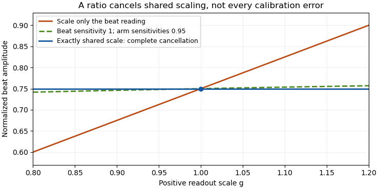
The physical calibration paths determine which model applies. NIST's receiver experiment combined two lasers through a beam splitter, polarizer and single-mode optical fiber, while separately correcting electrical loss and impedance mismatch.^[ref] An electronic gain change confined to the beat-frequency path need not appear in the arm-current measurements. Likewise, adding a current offset is not multiplication by a common factor. Background correction and the sharing of calibration factors must therefore be established before claiming cancellation.

Heterodyne amplitude-versus-power gain conversion translates a calibration of measured electric power into a calibration of beat-current amplitude. In a fixed resistive load, power is quadratic in current amplitude, so a multiplicative power correction becomes a square-root amplitude correction. The electrical reference plane and peak-versus-root mean square convention must also agree.

For sinusoidal load current $i(t)=B\cos \omega t$ and resistance $R$,For two measurements of the same load, $P_2/P_1=(B_2/B_1{)}^2$. A power multiplier of four therefore means an amplitude multiplier of two. In decibels, the same change is $10{\log }_{10}4=20{\log }_{10}2\approx 6.0206$ dB. NIST distinguishes the factor ten for power ratios from the factor twenty for field-amplitude ratios when their quadratic relationship applies.^[ref]

If the load resistance also changes, the more general relation isFor frequency-dependent complex impedances, use the appropriate circuit and power model rather than replacing resistance by an arbitrary complex number. A measured electric potential difference likewise requires its stated impedance before it can be converted to current.

For a corrected detector-current peak amplitude $B_d$, the normalized overlap is $\gamma =B_d/(2\sqrt{I_1{I}_2})$. If the numerator is instead detector-current RMS amplitude, the denominator is $\sqrt{2I_1{I}_2}$. Using an RMS numerator with the peak denominator lowers the result by $1/\sqrt{2}$, a 3.0103 dB discrepancy under the amplitude-ratio convention. The mistake is a convention mismatch, not evidence of worse optical overlap.

Current-plane convention in heterodyne calibration is another independent issue. In an ideal matched Norton circuit, a source peak current $B_d$ splits equally between source resistance and equal load resistance $R$. Load peak current is $B_d/2$, so delivered power is $B_d^{2}R/8$, rather than $B_d^{2}R/2$. The factor depends on the specified equivalent circuit; real detector capacitance and interconnecting networks require their measured response.

NIST's two-laser receiver apparatus measures microwave power and separately corrects sensor calibration, network loss and impedance mismatch. Its matched optical modes make the modulation calculable, while the electrical corrections locate the power at the intended reference plane.^[ref] Record raw power, correction factors, reference plane, load, amplitude convention and DC-current calibration separately. Only then apply the gain-matching condition for heterodyne normalization.

A heterodyne RF-to-DC gain transfer check tests whether the calibration converting a beat-frequency measurement into current amplitude is compatible with the calibration of the separate arm currents. The gain-matching condition for heterodyne normalization involves amplitude gains, so an RF power gain cannot be substituted without conversion.

For corrected peak beat current $B$ and arm currents $I_1,I_2$, the normalized overlap is $\gamma =B/(2\sqrt{I_1{I}_2})$. Suppose an electrical model gives sinusoidal peak current $B$ through a known resistive load $Z$. Its average beat power isSource/load division and impedance corrections must already be included when relating that load current to the detector-current convention. A factor converting power is therefore square-rooted when converting amplitude.

Let measured RF power carry multiplicative factor $g_P$, while the arm currents carry factors $g_1,g_2$. Under this model,Cancellation requires $g_P=g_1{g}_2$. With one common DC current factor $g_{\mathrm{DC}}$, the condition is $g_P=g_{\mathrm{DC}}^2$, not $g_P=g_{\mathrm{DC}}$.

An original example takes $g_{\mathrm{DC}}=1.10$. An RF power factor 1.21 produces amplitude factor 1.10 and cancels in the normalized overlap. Applying RF power factor 1.10 instead leaves multiplier $1/\sqrt{1.10}\approx 0.95346$, despite using the same numerical gain label in both paths. The example isolates heterodyne amplitude-versus-power gain conversion, rather than a change of optical overlap.

NIST's receiver experiment measured microwave power and separately corrected sensor calibration, electrical loss and impedance matching. Its two-laser optical source used polarization and spatial matching to establish calculable modulation.^[ref] Those separate operations make the RF-to-DC comparison a physical calibration problem.

Record peak versus RMS conventions, frequency response, load model and arm-current calibration. Test a known or independently characterized modulation while varying power within the linear range. Changed polarization, aperture clipping or optical alignment can alter the true overlap and imitate a gain-transfer defect, so one unexplained normalized ratio does not uniquely diagnose the electrical path.

Uncertain variance in heterodyne lognormal bias correction matters when a measured overlap is corrected using an estimated, rather than known, logarithmic variance. The known-variance correction is a nonlinear function of that estimate, so replacing the variance by an unbiased estimate does not automatically preserve unbiasedness of the corrected overlap.

Suppose $\hat{\gamma }=\gamma e^d$, with $d\sim N(0,v)$, and use $\tilde{\gamma }=\hat{\gamma }{e}^{-\hat{v}/2}$. If the variance estimate is independent of the overlap readout,Even if $\mathbb{E}[\hat{v}]=v$, Jensen's inequality gives $\mathbb{E}[e^{-\hat{v}/2}]\ge e^{-v/2}$. Consequently the mean corrected estimate is at least $\gamma$ under these independence and unbiased-variance assumptions. Equality requires a nonrandom variance estimate in the ordinary finite-variance case.

An original exact example uses a variance estimate from an independent normal calibration sample, with $\nu \hat{v}/v$ following a chi-squared distribution with $\nu$ degrees of freedom. Its Laplace transform givesThe logarithm of this factor is $v/2-(\nu /2)\log (1+v/\nu )$, which is positive for $v>0$. With stipulated $v=1$ and $\nu =2$, the factor is $e^{1/2}/1.5\approx 1.09915$: about a 9.91% remaining mean shift. This intentionally broad statistical example is not a typical receiver specification.

For fixed $v$ and large $\nu$, the logarithm is $v^2/(4\nu )+O({\nu }^{-2})$. More independent calibration information reduces this effect. Merely taking more overlap readings while retaining the same uncertain variance estimate does not remove its influence.

Dependent variance correction in heterodyne normalization requires the joint quantity $\mathbb{E}[e^{d-\hat{v}/2}]$ instead of the product of expectations above. A variance inferred from the same readout cannot simply be declared independent. Propagate the joint calibration and readout model, with a stated target summary. JCGM 101 treats input distributions from prior uncertainty calculations and numerical propagation explicitly.^[ref]

The optical gain-matching condition for heterodyne normalization still concerns physical calibration paths. This calculation addresses the statistical correction of residual log-errors; it does not imply that an imperfect RF or DC calibration can be repaired solely by subtracting a fitted variance.