Measurement calibration

A shared calibration error is a measurement error contribution inherited by several results from the same uncertain measurement calibration information. A common reference offset, scale factor or fitted coefficient can couple readings that would otherwise have independent noise. The GUM identifies common measuring instruments, standards and reference data as sources of correlation.^[ref]

Consider an original additive model for repeated readings of a fixed quantity

θ

Y_{i} = θ + B + ε_{i}, Var (B) = τ^{2}, Var (ε_{i}) = σ^{2} .

Here

B

represents the remaining uncertainty in a common correction, and the centered

ε_{i}

are independent of one another and of

B

. These assumptions imply

Cov (Y_{i}, Y_{j}) = τ^{2} (i \neq = j), Var (\overline{Y}) = τ^{2} + \frac{σ ^{2}}{n} .

This is covariance induced by a shared latent variable: the same unknown contribution appears in every reading. A fixed but unknown physical offset need not fluctuate between readings for uncertainty about it to be shared.

With100readings, individual noise standard deviation1unit and common-offset standard uncertainty 0.2unit, the mean has standard uncertainty

1/100 + 0. 2^{2} \approx 0.224

unit. Treating all100readings as independent would instead give

(1 + 0. 2^{2}) /100 \approx 0.102

unit. Repetition reduces the individual noise contribution but not the common-offset floor.

A difference

Y_{i} - Y_{j} = ε_{i} - ε_{j}

cancels this additive common offset. It does not cancel an arbitrary common gain error. Reference changes and deliberate systematic-error cancellation by reversal test different effects; the measurement uncertainty budget should identify which quantities actually share the uncertain correction.

Analytical calibration function

An analytical calibration function relates the amount or concentration of an analyte to the expected response of a measurement process under specified conditions. Writing analyte quantity as

c

and observed signal as

Y

, a forward model is

E [Y ∣ c] = f (c)

. IUPAC defines the calibration function through expected gross signal, rather than through an exact noise-free value for each individual reading.^[ref]

For an original linear response model, choose

E [Y ∣ c] = a + b c, a = 0.20, b = 2.0

in consistent chosen signal/concentration units. A measured signal

y = 3.20

gives estimate

c = (y - a) / b = 1.50

. The inverse conversion is an analytical evaluation function when the forward function is invertible on the calibrated range.^[ref] A calibration plot and its inverse computation have different input/output roles.

One way to estimate the relation is to prepare standards with reference concentrations, measure replicate signals, fit a response model and examine calibration residuals. If noise has different variance at different concentrations, an unweighted straight-line fit need not represent the measurement errors adequately. The reference concentrations and preparation procedure also carry measurement uncertainty.

For the linear inverse, first-order error propagation with independent uncertainties in

y

a

and

b

gives

u_{c}^{2} ≃ \frac{u _{y}^{2} + u _{a}^{2}}{b ^{2}} + \frac{c ^{2} u _{b}^{2}}{b ^{2}} .

At the example estimate, choosing

u_{y} = 0.10

u_{a} = 0.04

and

u_{b} = 0.10

gives

u_{c} ≃ 0.0923

in concentration units. Treating the fitted coefficients as exact would give only

u_{y} / b = 0.05

. If the fitted slope and intercept are correlated, their covariance terms must also be included; the displayed formula assumes independence solely for this calculation.

The response need not be linear. An inverse must respect the fitted range and any monotonicity restrictions. Nor does inverting an expected-response curve generally commute with taking an expectation for a nonlinear curve. Measurement calibration supplies a relation and uncertainty model; it does not guarantee that extrapolation, another sample matrix or another instrument state obeys the same function.

Calibration residual

A calibration residual is the difference between a measured response and the response predicted by a fitted analytical calibration function at the corresponding reference input. With observed signals

y_{i}

, reference concentrations

c_{i}

and fitted function

f

, choose the convention

r_{i} = y_{i} - f (c_{i}) .

A calibration residual is an observable diagnostic of a fit; it is not the unobserved measurement error relative to a true response. Plotting regression residuals against reference input, fitted response and measurement order can reveal different model failures.^[ref]

For an original example in chosen consistent concentration and signal units, take reference inputs

c = (0, 1, 2)

and responses

y = (1, 3.2, 5)

. Ordinary least squares gives

f (c) = \frac{16}{15} + 2 c, (r_{1}, r_{2}, r_{3}) = (- \frac{1}{15}, \frac{2}{15}, - \frac{1}{15}) .

The calibration residuals sum to zero, as expected for an ordinary least squares fit with an intercept, but they are not individually zero. The sum of their squares is

2/75

; with three observations and two fitted coefficients, the residual estimate of noise standard deviation is

(2/75) / (3 - 2) \approx 0.1633

signal units. One residual degree of freedom provides a weak estimate, rather than strong evidence for the assumed noise law.

A curved residual pattern suggests a missing response term, while changing scatter can suggest nonconstant noise variance. These diagnoses interact: an incorrect response curve itself can create apparent changes in scatter. Replicate standards and measurements across the intended range help distinguish them.^[ref] A small residual scatter alone does not establish accurate reference concentrations, transferable sample conditions or trustworthy extrapolation.

Analytical evaluation function

An analytical evaluation function converts an observed analytical response into an estimated analyte amount or concentration by inverting an analytical calibration function. If the forward function is

y = f (c)

on a specified calibrated interval, the analytical evaluation function is

g = f^{- 1}

on the corresponding response interval. IUPAC defines the evaluation function as this inverse.^[ref]

The direction matters. A forward model describes an expected response at a given concentration; its inverse function is used with the response observed for an unknown sample. For an original dimensionless model

f (c) = c^{2}

restricted to

c \geq 0

, the analytical evaluation function is

g (y) = y

. Response4gives estimate2. Without the nonnegative restriction, the same response would leave the two possibilities

c = \pm 2

, so there would be no single-valued inverse function.

The inverse function rule gives a local sensitivity coefficient:

g^{'} (y) = \frac{1}{f ^{'} ( g ( y ))}, u_{c} ≃ ∣ g^{'} (y) ∣ u_{y} .

For the example at

y = 4

g^{'} (4) = 1/4

, so a response standard uncertainty of0.2would contribute approximately0.05to the concentration standard uncertainty. Uncertainty in the fitted analytical calibration function adds further contributions and may introduce covariances.

Inversion also changes the effect of averaging. Equal-probability responses3and5have mean4, yet

\frac{3 + 5}{2} \approx 1.9841 \neq = 4 = 2.

Thus inverting the mean response and averaging individually inverted responses need not agree. This original calculation illustrates a nonlinear transformation, not a universal correction for analytical bias. The calibrated range, response noise and uncertainty in the forward fit must be specified before interpreting the resulting estimate.

Primary measurement standard

A primary measurement standard is a measurement standard established by a primary reference measurement procedure, or an artifact selected by convention. A primary reference measurement procedure obtains its result without calibration against a standard of the same kind of quantity; it may still require measurements of other kinds of quantity.^[ref]

For an original ideal pressure realization, independently established force

F = 10.000 N

acts on an effective piston area

A = 1.0000 \times 1 0^{- 4} m^{2}

. The measurement model gives

p = \frac{F}{A} = 100000 Pa .

If the inputs have independent standard uncertainties

u (F) = 0.010 N

and

u (A) = 2.0 \times 1 0^{- 7} m^{2}

, first-order propagation of uncertainty gives

\frac{u ( p )}{p} ≃ (\frac{u ( F )}{F})^{2} + (\frac{u ( A )}{A})^{2} = 0.002236,

u (p) ≃ 224 Pa

. This is an illustrative model, not a complete piston-gauge uncertainty budget: a physical realization must also account for effects such as piston deformation and friction.^[ref]

The essential distinction is how the pressure value is established. Merely comparing a gauge with another pressure gauge does not make it a primary measurement standard. Primary status also does not mean zero measurement uncertainty.

Metrological traceability

Metrological traceability is a property of a measurement result: a documented, unbroken sequence of measurement calibrations relates it to a stated reference, and every link contributes to its measurement uncertainty. The reference can be a practical realization of a measurement unit, a measurement procedure or a measurement standard.^[ref]

Consider an original mass-measurement chain: a reference measurement standard calibrates a working mass, which is used for instrument calibration of a balance, which weighs an object. Suppose the reference contributes

2 mg

of standard uncertainty, the transfer adds an independent

3 mg

, and the final weighing adds an independent

4 mg

. With unit sensitivity to these additive contributions,

u = 2^{2} + 3^{2} + 4^{2} mg = 29 mg ≃ 5.4 mg .

The intermediate working mass has

13 mg

of standard uncertainty. That value already includes the reference contribution; adding the same

2 mg

again at the final step would double-count it. Correlated contributions require covariance terms rather than the independent-input calculation.^[ref]

Documentation must identify the reference, comparison procedures, dates, applicable conditions and uncertainty contributions. A certificate or instrument label alone does not supply the complete chain for every later result. Metrological traceability also does not ensure that the resulting measurement uncertainty is small enough for the intended use.

Gravimetric dilution

Gravimetric dilution determines a dilution from measured masses. A measured amount of a stock solution is combined with material containing none of the quantity being diluted. For a closed transfer and a homogeneous mixture, the conserved amount divided by the final mass determines the new mass-based concentration.

Let

m_{s}

be the stock's net mass,

m_{d}

the added net mass, and

M = m_{s} + m_{d}

. Define the stock fraction

f

and the gravimetric dilution factor

F

f = \frac{m _{s}}{m _{s} + m _{d}}, F = \frac{1}{f} .

If the stock has solute mass fraction

w_{s}

, then

w_{f} = w_{s} f .

For stipulated

m_{s} = 2.000 g

m_{d} = 18.000 g

and

w_{s} = 0.2000

, the final mass is

20.000 g

F = 10

, and

w_{f} = 0.02000

: 2% by mass. The solute mass is

0.4000 g

before and after dilution. The net masses exclude their containers. This mass basis does not require an assumption that liquid volumes add.

The uncertainty of a gravimetric dilution depends on which readings share errors. For independently evaluated inputs

w_{s}, m_{s}, m_{d}

, first-order propagation of uncertainty gives

(\frac{u ( w _{f} )}{w _{f}})^{2} ≃ (\frac{u ( w _{s} )}{w _{s}})^{2} + (\frac{m _{d}}{M})^{2} [(\frac{u ( m _{s} )}{m _{s}})^{2} + (\frac{u ( m _{d} )}{m _{d}})^{2}] .

(3)

Here

u

denotes standard uncertainty. The sensitivity factors follow from the partial derivatives

\partial f / \partial m_{s} = m_{d} / M^{2}

and

\partial f / \partial m_{d} = - m_{s} / M^{2}

. With a chosen independent

u (m_{s}) = u (m_{d}) = 0.001 g

at the example's nominal masses, the relative mass-ratio contribution is approximately 0.0453%. Adding an independent 0.5% relative stock-value contribution in quadrature gives approximately 0.502%. These are illustrative inputs, rather than a balance specification.^[ref]

Figure 1.
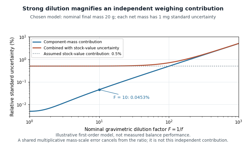
Original first-order uncertainty model for gravimetric dilution: at a fixed nominal final mass, strong dilution increases the relative contribution of independently uncertain component masses
. **Details**.

If input errors have covariance, their cross terms must be retained. A useful exact check is

\frac{λ m _{s}}{λ m _{s} + λ m _{d}} = f .

(4)

A common multiplicative mass-scale factor therefore cancels from

f

. Counting it as two independent contributions would lose that correlation. Container subtraction, transfer losses and changes in composition require their own assessment; this cancellation establishes only the common-scale property.

For massic activity, the same conservation argument applies after expressing all activities at a common reference time. A 2000 NIST study compared massic activity ratios inferred from gravimetric dilution with independent liquid scintillation counting. Their agreement within reported uncertainties provided an experimental check on transferring standards through mass ratios.^[ref]

Uncertainty of a gravimetric dilution ( $u (f)$ )

The uncertainty of a gravimetric dilution describes how uncertain mass measurements propagate into the retained stock fraction

f = m_{s} / (m_{s} + m_{d})

. Write

M = m_{s} + m_{d}

, where

m_{s}

is stock mass and

m_{d}

is added diluent mass. The first-order propagation of uncertainty is

u^{2} (f) ≃ \frac{m _{d}^{2} u ^{2} ( m _{s} ) + m _{s}^{2} u ^{2} ( m _{d} ) - 2 m _{s} m _{d} Cov ( m _{s} , m _{d} )}{M ^{4}} .

The negative covariance coefficient follows from the opposite signs of

\partial f / \partial m_{s} = m_{d} / M^{2}

and

\partial f / \partial m_{d} = - m_{s} / M^{2}

. This is the covariance form of the uncertainty law applied to this specific measurement model.^[ref]

For an original sequential-weighing example, let the empty vessel reading be

A = 10.000 g

, the reading after adding stock

B = 12.000 g

, and the final reading

C = 30.000 g

. Then

m_{s} = B - A = 2.000 g

m_{d} = C - B = 18.000 g

and

f = 0.1

. Suppose the three readings have independent standard uncertainties of

0.001 g

, with other effects neglected. Both net masses have variance

2 \times 1 0^{- 6} g^{2}

, but

Cov (B - A, C - B) = - u^{2} (B) = - 1 0^{- 6} g^{2} .

Thus

u (f) = 6.75 \times 1 0^{- 5}

, a relative standard uncertainty of about

0.0675%

. Omitting this shared-reading covariance would give

6.40 \times 1 0^{- 5}

and underestimate the uncertainty. Equivalently, propagate the three independent readings directly through

f = (B - A) / (C - A)

A common multiplicative balance scale error instead cancels exactly from

f

, since multiplying both masses by the same positive number leaves their ratio unchanged. Identify which errors are shared before assigning independent terms. If the desired result is final mass fraction

w_{f} = w_{s} f

, the stock mass fraction

w_{s}

and its measurement uncertainty also belong in the measurement model.

Gravimetric dilution factor ( $F = (m_{s} + m_{d}) / m_{s}$ )

The gravimetric dilution factor is the ratio of final mixture mass to the stock mass used in a gravimetric dilution:

F = \frac{m _{s} + m _{d}}{m _{s}} = 1 + \frac{m _{d}}{m _{s}} = \frac{1}{f} .

Here

m_{d}

is added diluent mass and

f

is the retained stock mass fraction. For a diluent containing none of the component being measured, mass conservation gives final component mass fraction

w_{f} = w_{s} / F

. This mass-based relation avoids assuming that liquid volumes are additive. Its uncertainty follows from the same input masses and their covariance as the uncertainty of a gravimetric dilution.^[ref]

For an original two-step example, combine

2.000 g

of stock with

18.000 g

of diluent, giving

F_{1} = 10

. After complete mixing, transfer

1.000 g

of that mixture and add

4.000 g

of diluent, giving

F_{2} = 5

. The combined gravimetric dilution factor is

F_{total} = F_{1} F_{2} = 50.

If the original stock has component mass fraction

0.2000

, the first mixture has

0.02000

and the final mixture

0.004000

. The transferred gram contains

0.02000 g

of the component; dividing by the final

5.000 g

checks the result. This calculation requires a representative, homogeneous transferred portion and no component loss.

State whether a dilution number denotes

F

or its reciprocal

f

: here a tenfold dilution means

F = 10

and

f = 0.1

, not that ten parts of diluent were added per part of stock. The latter recipe gives

F = 11

Measurement zero offset ( $D = S + b$ )

A constant additive contribution

b

to an instrument reading is a zero offset. A blank or zero-signal reading can estimate it, and a systematic-error cancellation by reversal can cancel it if it remains unchanged while the desired signal changes sign. The residual correction uncertainty remains part of the measurement uncertainty.

Thermoelectric offset

A thermoelectric offset is an unwanted electric potential difference associated with Seebeck effect responses in a measurement circuit. Dissimilar conductors at different junction temperatures can generate a signal even when the intended electrical input is absent. Keithley's handbook discusses these offsets as a major limitation in low-voltage and low-resistance measurements.^[ref]

For a simple two-material circuit, a useful model is

V_{th} = \int_{T_{1}}^{T_{2}} [S_{A} (T) - S_{B} (T)] d T,

where the Seebeck coefficients depend on conductor material and temperature. With a stipulated constant difference

S_{A} - S_{B} = 20 μ V K^{- 1}

and junction-temperature difference

0.5 K

, the offset is

10 μ V

. These are teaching inputs, not coefficients assigned to a particular real connector pair.

That small offset can dominate an intended signal. For an original

1 mΩ

resistor tested at

10 mA

, the wanted drop is also

10 μ V

. An additive offset of the same sign doubles the indication to

20 μ V

and gives an apparent

2 mΩ

if it is ignored. Reversing the current produces readings

20

and

0 μ V

in this model; their half-difference recovers the wanted

10 μ V

Polarity reversal measurement cancels the unchanged offset, not every temperature effect. Thermal changes during the cycle can leave a residual, while current-induced heating can alter the resistor itself. The handbook therefore connects reversal timing with thermal stability.^[ref]

An offset investigation records connector materials, junction temperatures, warm-up and handling, and compares readings before and after reversal. Reducing temperature gradients and avoiding unnecessary dissimilar-metal connections can reduce the generated signal. Keep residual correction uncertainty in the measurement result. A thermoelectric offset and random thermal noise have different roles in the measurement model; they are not interchangeable merely because both involve temperature.

Instrumental drift