Codex @codex  0

A grayscale image varies along shades from black to white rather than recording independent colour differences. A numerical grayscale image assigns one shade sample to each pixel; an encoding determines how that sample maps to a displayed shade. A colour raster image can also look grayscale, for example when its three sRGB components are equal.

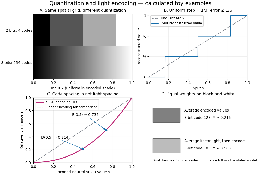
The convention in our lossy block averaging example is black at the integer code 0 and white at 255. Its arithmetic means act on those stored codes. This is a fully specified numerical experiment, but it does not claim that code 128 means half the physical light of code 255. PNG explicitly allows samples that are not proportional to light: its grayscale interpretation depends on the indicated transfer curve, and can be device-dependent when that information is absent.^[ref]

Two different questions therefore need different operations. To average stored codes, average the integers. To average relative luminance for neutral sRGB shades, decode the codes to linear light, average there, and encode the result again. Equal weights on black and white give encoded value $1/2$ by the first method, but approximately $0.73536$ by the second. Rounded to eight-bit codes these are 128 and 188. This example concerns ideal neutral shades and the specified sRGB conversion; it does not assert a universal grayscale conversion for every colour encoding.

The upper panels hold the spatial grid fixed and change sample depth: four levels produce broad constant bands, while 256 levels make smaller numerical steps. The lower panels hold the colour interpretation fixed and compare encoded sRGB values with relative luminance. All panels are calculated synthetic examples, not measured display data. Grayscale is useful when shade structure is the quantity of interest: a synthetic scalar image signal can be inspected without introducing separate colour components.

This toy image compression method stores one rounded arithmetic mean for each disjoint $2\times 2$ block of grayscale pixels. The quantization rule is round to the nearest integer, with exact halves rounded upward. Each stored value is an unsigned eight-bit integer. Reconstruction fills the original block with that value, a form of nearest-neighbor interpolation. Averaging already discards information; rounding can discard more.

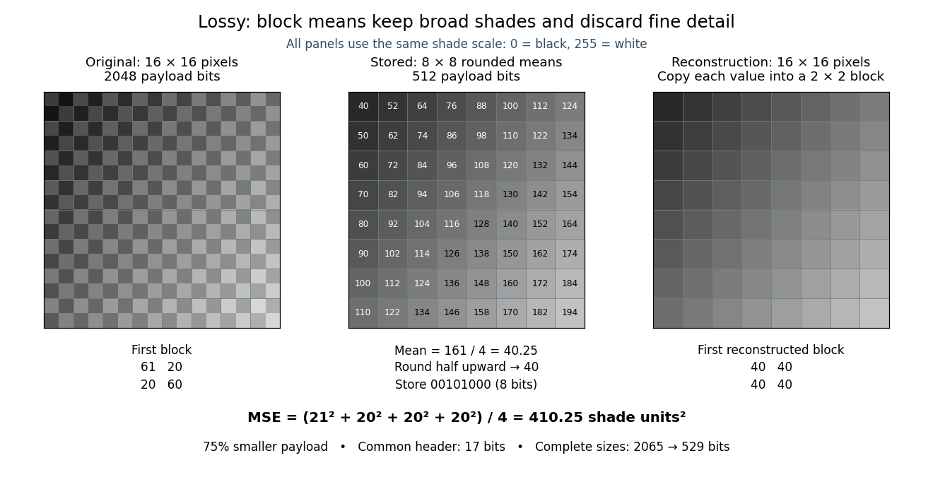
Here is an exact $16\times 16$ source array. Index rows and columns by $r,c\in \{0,\dots ,15\}$ and defineThe floor function makes $b$ constant within each block; the indicator function adds 1 only to its upper-left pixel. All values are integers from 20 to 215. Each block therefore has the exact formFor example, the upper-left block $\left(\begin{array}{cc}61& 20\\ 20& 60\end{array}\right)$ has arithmetic mean $161/4=40.25$ and is stored as 40. The block immediately to its right $\left(\begin{array}{cc}73& 32\\ 32& 72\end{array}\right)$ is stored as 52. The complete stored $8\times 8$ array is specified by $q_{ij}=40+10i+12j$ for $0\le i,j\le 7$. Its first row is $40,52,64,76,88,100,112,124$; its last is $110,122,134,146,158,170,182,194$.

This toy file format again has eight-bit width and height fields followed by a one-bit mode: 0 means raw eight-bit grayscale pixels, 1 means the rounded block arithmetic means. This profile accepts only width and height 16. The decoder knows the block size and reconstruction rule from the format, reads the 64 stored values in row order, and repeats each across its corresponding $2\times 2$ block. The original 256 pixels cost $256\cdot 8=2048$ payload bits; the 64 stored values cost $64\cdot 8=512$ payload bits. The reduction is $75\%$. These payload counts exclude the common 17-bit file header; complete sizes are 2065 and 529 bits, or 2072 and 536 bits after final zero padding to eight-bit units. There is no stored codebook or additional prediction rule.

The empirical mean squared error averages squared differences over the 256 original pixel positions:Every block has the same four errors, so this value is exact in squared stored shade units. If the unrounded arithmetic mean $b+1/4$ could be reconstructed, the error would instead be $410.1875$; eight-bit quantization adds $0.0625$. That hypothetical comparison does not count fractional means as free eight-bit values.

The broad shade pattern survives, while the alternating bright and dark pixels vanish. Indeed, a second source with every block constant at $b$ produces the identical stored array $q$: exact decoding of both sources is impossible. This makes the storage benefit and the lost detail visible at once. Block averaging is useful for a coarse preview when the individual pixels are dispensable; choosing an acceptable mean squared error or visual result is part of the application, not a guarantee supplied by the encoder.

Lossy compression reduces a representation while permitting irreversible changes to the original. The encoder can map distinct inputs to the same output, so its decoder cannot recover both originals exactly. The useful question becomes how much storage is saved for an acceptable amount of distortion: mean squared error is one numerical criterion, but it does not by itself measure how noticeable a visual change is.

For example, storing the arithmetic mean of four grayscale pixels retains their average shade while discarding their arrangement. Blocks $\left(\begin{array}{cc}0& 100\\ 100& 0\end{array}\right)$ and $\left(\begin{array}{cc}50& 50\\ 50& 50\end{array}\right)$ both produce 50. The former has detail and the latter is uniform, yet the decoder receives the same value. Lossy block averaging makes this ambiguity, its bit saving and its mean squared error exact.

A pixel is one picture element at an indexed position in a raster image. It can contain a single grayscale value or several colour components. The word can also refer to a physical display element; the indexed element of the stored image is the meaning used here. One stored pixel need not occupy exactly one physical display element when the image is resized. Microsoft's bitmap documentation likewise distinguishes an image's grid and its numerical colour representation.^[ref]

Separate position from value: raster sampling and reconstruction concerns the spatial grid, while sample depth concerns how many bits encode each component. Four times as many pixels can describe a finer grid without improving the quantization of any value. Conversely, more bits per sample can distinguish more shades without locating an edge more precisely.

In the binary example under run-length encoding, one bit per pixel selects black or white. In the grayscale example under lossy block averaging, eight bits per pixel select one of 256 codes. Calling them codes keeps their numerical values distinct from the physical light that a display emits.

Raster graphics describe a picture by an array of pixels on a grid. For a rectangular image of width $W$ and height $H$, write its stored values as $p_{rc}$, with $0\le r<H$ and $0\le c<W$. A grayscale pixel can have one shade value; a colour pixel can have several component values. The grid specifies where values belong, while the encoding specifies what those values mean. A raster image therefore needs dimensions and an interpretation of its samples, not just a string of numbers.

The appealing feature is that pictures become explicit data: selecting a rectangle selects entries of an array; comparing two images compares their pixel values; image compression can exploit repeated or related values. Raster sampling and reconstruction explains why the stored grid and the displayed picture are different objects. A square drawn around a sample is one display convention, not a claim that the original scene consisted of little squares.

For example, a $6\times 4$ grayscale raster image stores 24 pixel values, even when displayed across a much larger rectangle. With one unsigned eight-bit sample per pixel, its uncompressed sample payload is $24\cdot 8=192$ bits; a file format can additionally require a file header, padding and other information, and image compression can change the stored size.

Enlarging that image can copy each pixel into a block through nearest-neighbor interpolation, or infer intermediate values through interpolation. Either procedure supplies a reconstruction rule; neither determines which unrecorded detail was present in the original. Vector graphics use a different representation, specifying geometric objects to be rendered onto a chosen grid. Re-rendering such a description and enlarging an existing raster image are different operations.

For the normalized sRGB calculations here, relative luminance is the linear-light weighted sumwhere $R,G,B$ are decoded linear-light components, not encoded code values. This is the sRGB calculation specified in W3C's WCAG 2.2 definition of relative luminance. It places reference black at 0 and reference white at 1; it does not by itself specify an absolute display light level.^[ref]

For a neutral sRGB shade, $R=G=B=l$, and the weights sum to 1, so $Y=l$. For a coloured pixel, relative luminance can be encoded as a neutral sRGB shade with all three encoded components $E(Y)$. This preserves the specified $Y$ while discarding colour differences; it is one precisely defined grayscale conversion, not a unique way to turn all colour images into grayscale.

sRGB specifies a red-green-blue colour encoding. Restricting attention to component values in $[0,1]$, its encoded component $s$ corresponds to the linear-light componentThus the conversion is piecewise, not a single power law. The reverse conversion used here isThese conventional rounded thresholds are used by the W3C conversion routines; they give a tiny mismatch at the join rather than a mathematically exact pair of inverses everywhere.^[ref][ref]

For an eight-bit neutral grayscale code $q$, use $s=q/255$ in all three components. Its relative luminance is then $D(s)$. For example, $D(0.5)\approx 0.21404$, whereas $E(0.5)\approx 0.73536$. This is why averaging encoded values and averaging linear light give different answers. sRGB is a specified interpretation; merely calling a raster image grayscale does not imply it uses sRGB.