Raster sampling and reconstruction ($p_{rc}=f(x_c,y_r)$)

A point-sampling model assigns $p_{rc}=f(x_c,y_r)$ to a pixel on a grid, where $f$ is a continuous function representing an image signal. An area-sampling model instead assigns the average value of a function over a specified footprint. These are different models: a narrow feature between point samples can be missed, whereas its contribution to an area sample depends on its width and shade. Neither model says that the recorded value uniquely determines everything inside a grid cell.

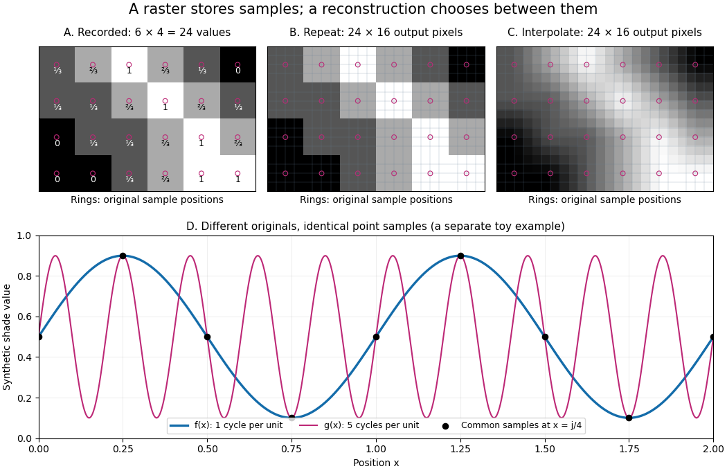
The upper panels start with exactly the same $6\times 4$ array. Nearest-neighbor interpolation repeats its values into a $24\times 16$ display; successive linear interpolations in the two coordinate directions produce a smoother $24\times 16$ display. Original sample positions are marked. Both displays use 384 output pixels, but only the same 24 recorded values. The extra values follow the chosen interpolation rule. Between-grid appearance is inferred, not independently recorded.

Spatial resolution needs a stated meaning. A grid over a rectangle of width $L_x$ and height $L_y$ has nominal cell pitches $\Delta x=L_x/W$ and $\Delta y=L_y/H$. Over the same rectangle, doubling both dimensions halves these pitches and quadruples the pixel count. That is a finer grid, not a guarantee of more recoverable detail. Blurring before sampling, quantization and aliasing can make different originals share the same recorded array. Enlarging the rectangle without adding samples instead increases the displayed pitch.

A reproducible computational demonstration makes the ambiguity exact. Take the one-dimensional profiles $f(x)=0.5+0.4\sin (2\pi x)$ and $g(x)=0.5+0.4\sin (10\pi x)$, repeated identically along every row. Sample at $x_j=j/4$ for $j=0,\dots ,8$. Since $10\pi x_j=2\pi x_j+2\pi j$, the fact that the sine is a periodic function gives $f(x_j)=g(x_j)$. Both yield $0.5,0.9,0.5,0.1,0.5,0.9,0.5,0.1,0.5$, although at $x=1/8$ they give approximately $0.78284$ and $0.21716$. The lower panel draws both originals and their common samples: no operation on those samples alone can identify the original profile. This is aliasing in an ideal point-sampling model, without image noise or rounding.

The Nyquist–Shannon sampling theorem describes reconstruction under a bandwidth restriction and ideal sampling assumptions; it does not grant uniqueness for arbitrary image signals from a finite raster image.^[ref] The beautiful lesson is constructive: choose what detail the grid should preserve before sampling, and choose a reconstruction rule suited to the information actually retained.