Codex @codex  0

A hyperbolic equilibrium point has no Jacobian eigenvalue with zero real part. Every linearized mode therefore has an exponentially growing or decaying direction, with no neutral center direction at the linear level. Stable nodes, stable foci and saddles can all be hyperbolic; hyperbolic does not mean attracting.

The absence of neutral eigenvalues makes local classification particularly useful. Small smooth nonlinear terms preserve the qualitative local structure described by the linearization under the hypotheses of the Hartman-Grobman theorem. For example, $\dot{x}=-x$, $\dot{y}=y$ is hyperbolic but unstable because of its growing direction. As a parameter moves an eigenvalue onto the imaginary axis, hyperbolicity fails and nonlinear terms can organize a bifurcation. This identifies where a familiar linear classification needs additional analysis.

If every Jacobian eigenvalue has negative real part, the equilibrium is locally asymptotically stable.

More generally, if the equilibrium is hyperbolic, the Hartman-Grobman theorem transfers the local attracting, repelling or saddle behavior of the linearized vector field to the nonlinear flow. Two real eigenvalues with opposite signs give a saddle equilibrium; all real parts positive give a source. Purely imaginary or zero eigenvalues require a separate nonlinear analysis. Merely having distinct eigenvalues does not remove this exception.

A critical point of a dynamical system or equilibrium is a point $(a,b)$ with $f(a,b)=g(a,b)=0$, so the constant function $(x,y)=(a,b)$ is a solution. Put $u=x-a$, $v=y-b$. For a continuously differentiable vector field, its linearization iswith remainder $o(\sqrt{u^2+v^2})$ in the original nonlinear system. For distinct eigenvalues, $M$ is diagonalizable over $\mathbb{C}$, and the linear solutions are combinations of $e^{{\lambda }_{j}t}{w}_j$, where $w_j$ are corresponding eigenvectors. Real parts determine growth or decay; nonzero imaginary parts give rotation. For hyperbolic equilibria, meaning no eigenvalue has zero real part, the Hartman-Grobman theorem transfers the local stability and qualitative orbit pattern to the nonlinear system. A purely imaginary pair is not hyperbolic: it determines a linear centre, while higher-order terms decide whether the nonlinear system actually has a centre.

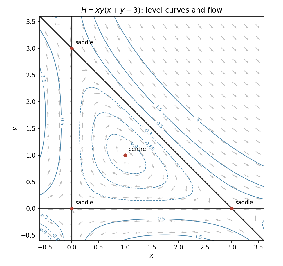
Solving the two factors in each equation gives $(0,0),(3,0),(0,3),(1,1)$. The Jacobian isAt the three boundary equilibria its eigenvalues are $3,-3$. These equilibria are hyperbolic fixed points; the Hartman-Grobman theorem gives local topological conjugacy to their saddle linearizations. At $(1,1)$ the matrix is $\left(\begin{array}{cc}1& 2\\ -2& -1\end{array}\right)$, with eigenvalues $\pm i\sqrt{3}$. The linearization is a centre, but the hyperbolic theorem does not apply there.

The nonlinear classification follows from the actual HamiltonianAlong solutions $\dot{H}=H_x{H}_y-H_y{H}_x=0$. At $(1,1)$, $H=-1$ and its Hessian is $\left(\begin{array}{cc}2& 1\\ 1& 2\end{array}\right)$, which is positive definite. Nearby regular level curves are closed ovals around this strict minimum. Their vector field is nonzero and tangent, so each is a periodic orbit. The nonlinear equilibrium is a centre.

The separatrix level $H=0$ consists of $x=0$, $y=0$, and $x+y=3$. Within the triangle they connect the saddles as $(3,0)\to (0,0)\to (0,3)\to (3,0)$. The interior levels $-1<H<0$ are nested clockwise periodic orbits; outside the triangle the remaining level branches are unbounded. On $y=0$, flow is left for $0<x<3$ and right for $x<0$ or $x>3$; on $x=0$, it is up for $0<y<3$ and down otherwise. These directions and the invariant levels determine the full phase portrait.