Kalman filtering of a moving scalar state ($P_t^{-}=P_{t-1}+Q,K_t=P_t^{-}/(P_t^{-}+R)$)

Consider a local-level state-space model $x_t=x_{t-1}+w_t$, $y_t=x_t+v_t$, with mutually independent centered Gaussian noises of variances $Q=1/4$ and $R=1$. Start with $x_0\sim N(10,4)$, independently of these noises. Before the first observation, the Kalman prediction step gives $m_1^{-}=10$, $P_1^{-}=17/4$. If $y_1=14$, the Kalman gain is $17/21$, and the posterior mean and posterior variance becomeThe next Kalman prediction step keeps the mean $m_2^{-}=278/21$ but adds fresh process noise variance, giving $P_2^{-}=89/84$. If $y_2=12$, thenThus new uncertainty is introduced at each transition and reduced by each measurement. It does not shrink to zero merely because many measurements have arrived: the state continues to change.

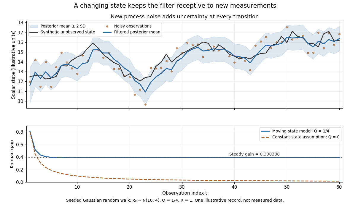
The steady-state local-level Kalman gain here isWith $R=1$, the limiting posterior variance has the same numerical value. By contrast, the static-state model $Q=0$ with $P_0=4$ gives $P_t=1/(t+1/4)$ and $K_t=1/(t+1/4)$. That decreasing gain is appropriate for a state that truly remains constant. Applied to the changing random walk, it builds confidence in the wrong model. The choice of process noise is therefore a statement about state evolution, rather than just an instruction to make a plot look smoother.