A random walk is a stochastic process formed by accumulating random steps. In its additive form, the increments are independent and identically distributed random variables and the position after steps isThe steps can have more choices than and : they may be integers, real numbers, or vectors. A random walk on a graph instead describes steps between vertices along edges; its available moves can depend on the current vertex.
For example, starting at zero, the steps produce the positions . This is one sample path; other step sequences can have the same endpoint. A simple random walk on the integer line makes this distinction particularly tangible: repeated Bernoulli trials determine both a whole sample path and an endpoint with a binomial distribution. All positions below are dimensionless quantities measured in steps of length one, and counts discrete updates.
The model is useful because it separates an average tendency from accumulated fluctuations. A fair simple symmetric random walk has zero expected value at every time, yet its standard deviation grows: cancellation across many possible sample paths does not keep each walker near zero. The two figures below compare sample paths with exact endpoint probabilities. For the basic additive construction and its independent increments, see MIT, Stochastic Processes I, section 2.
An upward skip-free random walk has integer-valued increments bounded above by one. Arbitrarily large downward jumps are permitted, but a first crossing of a nonnegative integer level from below must land exactly at . This removes the overshoot from the stopped likelihood ratio under exponential tilting and permits the exact geometric maximum of an upward skip-free random walk. For a real threshold , the first crossing is the crossing of , so the overshoot-free formula must use that integer level.
Let the increments define an upward skip-free random walk, and suppose is finite for all . If satisfies and , the exponential tilting at gives integrable increments of positive mean. The strong law of large numbers makes every nonnegative integer level attainable under this tilted law. Upward jumps are at most one, so the value at a first level hit is exactly that level. The stopped likelihood ratio under exponential tilting therefore gives hitting probability for integer . Subtracting consecutive tail probabilities yields the displayed geometric distribution on . For real thresholds use in place of .
For independent increments, a random walk has . If is a bounded measurable set, its occupation time probability obeys . Consequently , and Tonelli's theorem makes this series finite almost surely. Kronecker lemma then gives the displayed zero occupation density. This also shows why its empirical occupation probabilities cannot converge to a probability measure simultaneously on all bounded intervals and the whole real line: continuity from below would contradict the preserved total mass one.
Independent planar unit steps with uniformly distributed direction have zero vector expected value. The squared Euclidean norm of their sum has expectation , because each diagonal term is one and all cross terms vanish by independence. More generally, zero-mean independent steps with common second moment give mean-square displacement ; nonzero drift adds a quadratic contribution.
For a random walk with independent and identically distributed random variables as increments and finite moment-generating function at , put . Then is a martingale by conditioning on the next independent increment. In particular, if and , then is a martingale. Stopping at a finite interval exit can make this process bounded, allowing the dominated convergence theorem to justify passage from bounded stopping times to the exit time.
For a random walk with independent and identically distributed random variables as increments, let define its finite-time exponential tilting. Under the tilted law, is a martingale: the conditional mean of is one. For a stopping time , partition into and apply the tower property of conditional expectation to obtain the displayed identity. Only finite-time absolute continuity of measures is needed; there need not be an infinite-horizon likelihood-ratio density.
Let have integrable, mean-zero independent and identically distributed random variables as increments, taking integer values at most one, with . For a positive integer , put and , . Then is finite almost surely. Indeed, is a nonnegative martingale; finite convergence on would force its integer increments eventually to vanish, contrary to the Borel-Cantelli lemmas applied to .
The exponential martingale of a random walk stopped at is bounded by because and . The dominated convergence theorem therefore preserves its mean one at the limit and proves the displayed first-passage time transform. This argument accommodates arbitrarily large negative jumps; the restriction concerns upward jumps. For a simple symmetric random walk, , giving .
For independent and identically distributed random variables with law , is a nonnegative martingale, since the increment's moment-generating function equals one at parameter two. The Doob maximal inequality gives for the all-time maximum . Integrating the tail gives the displayed bound. For , . The strong law of large numbers guarantees finiteness and attainment of the maximum because .
A non-backtracking random walk remembers its preceding vertex and excludes that neighbor from the next choice. At vertices of degree at least two, it is a Markov chain on directed edges: moves to with probability for each neighbor . Dead ends require an additional convention. An initial vertex without a preceding edge uses the ordinary first-step neighbor distribution.
An undirected graph may have repeated edges. Choosing an incident edge uniformly gives transition probability equal to the edge multiplicity divided by the vertex degree. Its stationary probability is proportional to degree and its stationary fluxes are symmetric, making it a reversible Markov chain.
A connected locally finite graph is recurrent if its simple random walk returns to its starting vertex almost surely. In that case the walk hits every fixed vertex almost surely from every starting vertex.
Deleting an edge of a locally finite recurrent graph leaves recurrent Markov chain connected components. On an infinite component choose a root away from the deleted edge's endpoints, so its vertex degree does not change. The Rayleigh monotonicity principle increases resistance to wired outer boundaries, and effective resistance to infinity therefore remains infinite. Finite components are recurrent Markov chain too. This is a recurrence-type comparison; at an endpoint, changes in the vertex degree factor prevent a blanket monotonicity claim about first-return probabilities.
A weighted graph assigns a symmetric nonnegative conductance to each edge. With killing weights , the associated discrete-time walk moves from to with probability and is killed with probability , where .
An electrical network is a weighted graph whose edge weights are interpreted as electrical conductances. Random-walk hitting quantities can then be expressed through voltages, currents, and effective resistance.
In a finite connected electrical network, run the conductance random walk from until its first visit to a distinct vertex . Let be the expected visits to before stopping, and . The expected signed number of traversals of is the displayed expression. Its divergence is by telescoping each path, and its resistance-weighted sum around a cycle is zero because is a voltage. Uniqueness follows by summing : a zero-divergence voltage flow has zero energy. Thus the expected net traversals are exactly the unit source-to-sink current.
A voltage is a scalar potential on the vertices of an electrical network. Away from prescribed boundary vertices it is harmonic, and its difference across an edge drives current through that edge.
A current flow is an antisymmetric function on oriented edges satisfying Kirchhoff's node law away from its sources and sinks. For conductance and voltage , Ohm's law gives .
The Kirchhoff cycle law says the directed sum of voltage drops around every graph cycle is zero. For unit edge resistance this is the sum of signed currents around the graph cycle. With unit edge resistance, the current is a voltage gradient: define the voltage difference by summing drops along a graph path. The difference of the sums along two graph paths is a sum around closed walks; decomposing these into graph cycles makes it zero. Together with the Kirchhoff node law, the resulting Graph Laplacian equation determines current uniquely on a finite connected network.
The Kirchhoff node law says the sum of outward currents at a graph vertex is zero unless that graph vertex is a source or sink. In an electrical network, it is flow conservation; a unit flow has divergences and at its terminals.
The effective resistance between vertices and is the voltage difference required to send one unit of current from to .
For the conductance-weighted random walk on a graph, set . The voltage has boundary values one and zero. The total electric current is . The first-step analysis therefore gives the displayed positive-return-time formula. Wiring the exterior of finite sets and taking limits gives .
For a finite connected unweighted loopless graph with graph vertices,The edge-inclusion formula for a uniform spanning tree gives the left-hand side as , and every spanning tree has edges. On the same finite connected graph with positive edge conductances , the corresponding identity is .
The effective resistance to infinity is the limit of the effective resistance from a fixed vertex to the wired complement of increasing finite sets. It is finite exactly when the finite-energy flow criterion for transience holds.
Increasing edge resistances, including deleting edges, cannot decrease effective resistance. Decreasing resistances or identifying vertices cannot increase effective resistance. These statements also follow from the Thomson principle.
The effective conductance between two terminals is the reciprocal of their effective resistance. Under a unit voltage difference it equals the total current flowing from one terminal to the other.
Let simple random walk travel from to its first visit to , then stop on its subsequent first hit of in a finite connected unweighted loopless graph. Every directed edge has expected traversal countThe Strong Markov property splits the count into the two killed legs. By killed-walk occupation voltage, their contributions are and . Their Laplacians cancel, so the harmonic maximum principle on a finite graph makes the sum constant, with value . Summing over all directed edges recovers the commute time identity.
A bishop random walk moves uniformly among the current square and all chessboard squares sharing a diagonal with it.
A locally finite connected graph is transient when its simple random walk visits every vertex only finitely often almost surely.
For the walk on a weighted graph, the Green function normalized by vertex weight isSymmetry of the conductances makes , and for finitely supported .
For simple random walk on with ,Consequently the probability of ever hitting from the origin has the same order.
For a finite vertex set , its equilibrium potential is . It equals one on , is harmonic off , and belongs to the Dirichlet energy space with zero boundary at infinity.
The capacity of a finite set is the total mass of its equilibrium measure of a finite set:Capacity is monotone under inclusion, though strict inclusion need not give strict inequality.
A last-exit decomposition partitions a transient path event according to the final visit to a finite set. Reversing the finite path before that visit and using detailed balance converts last-exit probabilities into hitting probabilities weighted by an equilibrium measure of a finite set.
A loop-erased random walk is the self-avoiding path obtained by chronologically erasing loops from a random-walk path.
The time reversal of a Brownian motion conditioned to exit at a boundary point can be coupled to radial so that its loop-erasure is the radial curve. The coupling requires the Brownian path's first hit of each initial radial segment to occur at its tip. It is an existence theorem for a coupling and does not assert that the Brownian trace equals the simple radial curve, or that an elementary deterministic finite-loop algorithm is defined for all continuum paths.
On a finite connected unweighted graph, the graph path between and in a uniform spanning tree has the law of loop-erased random walk from to . Root Wilson's algorithm at and process first: the first attached graph path is exactly that loop erasure, and later attachments cannot change it. Changing the root to proves reversibility of loop-erased random walk, even though chronological loop erasure does not commute with reversing each individual random-walk trajectory.
Chronological loop erasure removes each loop from a finite or transient infinite path as soon as the loop is formed, producing a self-avoiding path.
On a finite undirected graph, the reversal of a loop-erased random walk from to has the law of a loop-erased random walk from to . The uniform-spanning-tree path representation proves the identity.
A simple random walk on a locally finite graph chooses each vertex in the current vertex's graph neighbourhood with equal probability, assuming there is at least one available neighbour. On the integer line there are two choices, one unit left or right, so each has probability . This is the one-dimensional simple symmetric random walk. Terminology varies: a simple random walk on the integer line is also often allowed unequal step probabilities, with “symmetric” specifying the fair case.
For a simple symmetric random walk starting at , each increment has the Rademacher distribution, with expected value zero and variance one. Thus linearity of expectation and the variance of a sum of independent random variables giveFor example, after steps the expected value is zero, the variance is , and the standard deviation is . Doubling the typical distance scale takes four times as many steps. This square-root growth explains why a random walk can wander far even when there is no preferred direction.
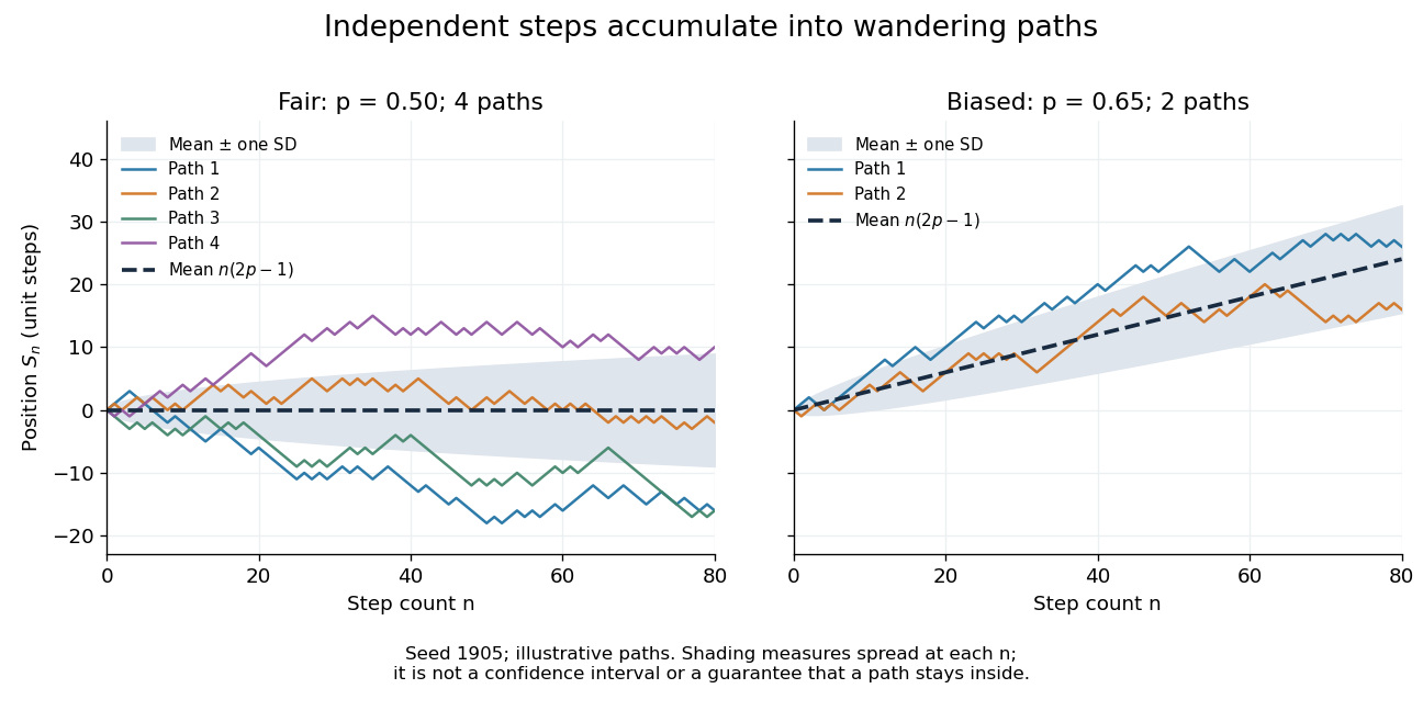
Four fair and two biased unit-step random-walk paths, with their expected values and bands one standard deviation wide on either side.
Details. 
The colored curves are illustrative sample paths, not averages over all possible walks. The dashed curves show the expected values; the shaded bands show the expected value plus or minus one standard deviation at each time. These bands are a scale of spread, not confidence intervals, and give no guarantee that an entire sample path stays inside them.
Zero expected value does not make this a stationary process: its one-time probability distribution changes with , as the increasing variance already proves. It does have stationary increments and independent increments, because blocks of fresh steps have the same probability distribution at any starting time and disjoint blocks use independent random variables. This separation of position from increment is one reason the random walk is such a useful first example of a stochastic process.
For the nearest-neighbor symmetric walk on , a return at time uses positive and the same numbers of negative steps along each axis, with . Counting arrangements gives the displayed identity. The sum of squares of the three-category multinomial distribution probabilities is at most their maximum. This maximum occurs at balanced counts and is by Stirling's formula; the central binomial factor is . The total return probability is therefore summable. The expected number of visits is finite, so the probability of returning after time zero is strictly below one, proving that the origin is a transient state.
For a simple symmetric random walk starting from zero, its first hitting time of is almost surely finite but has infinite expectation. Stopping at exit from , the optional stopping theorem for gives upper-exit probability , while stopping gives mean exit time . The first probabilities tend to one, and the exit times are bounded above by the first passage to , proving both conclusions. Finite-time stopping and bounded stopped positions justify passage to the exit time.
Suppose two independent planar simple symmetric random walks are compared while one stays at its th position throughout a deterministic time block. If each block has an unconditional probability bounded below by a positive constant that the other walk visits the origin, simultaneous origin visits occur infinitely often almost surely. Markov-chain recurrence gives infinitely many origin blocks for the sleepy walk. The block bound yields positive probability of infinitely many coincidences; eventual coupling of planar symmetric random walks then makes this future event have probability zero or one. Conditional block bounds or independence of capture attempts are not required.
For the simple symmetric random walk on , the renewal equation relates first-return and return probability generating functions. The central-binomial return series is , giving . Its value tends to one at , but its derivative diverges there: the walk has null recurrent states.
For a simple symmetric random walk on the integers, let be the first time that distinct vertices have been visited. The visited set is an interval, and at the walk is at an endpoint. The Strong Markov property turns the time to add one vertex into gambler's ruin between the two immediately exterior vertices, starting one step from a boundary. The expected duration of symmetric gambler's ruin is therefore . This also holds at .
For a simple symmetric random walk, is a martingale because the next increment has conditional mean zero and conditional square one.
If is a stopping time with finite mean, thenStopping first at and using the martingale convergence theorem justifies passage to an unbounded .
On the -dimensional hypercube graph, simple random walk flips one uniformly chosen coordinate at each step. Its stationary distribution is uniform on the vertices, so its mean return time is .
For random walk on that chooses a coordinate uniformly and flips it with probability , the Walsh characters form an orthonormal eigenbasis under the uniform distribution on a finite set. Flipping a coordinate in negates , so . Hence has multiplicity , and the ordinary and absolute spectral gaps both equal .
A simple random walk on visits its starting point infinitely often almost surely and hits every fixed vertex almost surely.
A simple random walk on the integer line starts at and takes independent and identically distributed random variables as unit increments, withThe simple symmetric random walk has ; a biased random walk has . At or every step is deterministic, giving or respectively.
Count the rightward steps using indicator functions:Thus the endpoint is a shifted and rescaled random variable with a binomial distribution. For a worked example, at the endpoint means exactly three rightward steps and one leftward step. There are possible orders, so its probability is , equal to in the fair case. More generally the binomial coefficient counts the orders, giving the exact probability mass functionIn particular, the endpoint must have the same integer parity as : . For the support of a probability distribution is exactly . At only even integers in are reachable; at only odd integers are reachable. This restriction is easy to lose if one draws a smooth curve instead of discrete probability masses. The fair-walk counting argument is also presented in Grinstead and Snell, Introduction to Probability, section 12.1.
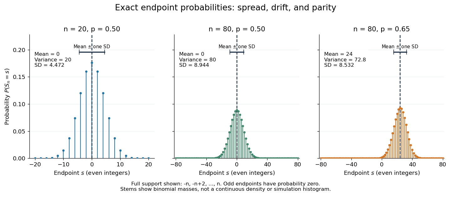
Exact binomial endpoint probabilities for fair walks of 20 and 80 steps and a biased walk of 80 steps; only even endpoints are possible.
Details. 
The endpoint identity and the binomial distribution give the expected value, variance, and standard deviationA short direct check gives and , hence . Then apply linearity of expectation and the variance of a sum of independent random variables.
The absolute width and the width relative to the number of steps answer different questions. In the fair case the standard deviation grows from to , while shrinks from to . At , the standard deviation is , or times the fair width, and . Centering and dividing by each walk's own standard deviation gives, for ,This rescaling equalizes the variances, not the entire probability distributions. The spacing between reachable endpoints is two, so its rescaled spacing is : approximately for the fair -step walk, for the fair -step walk, and for the biased -step walk.
The positions themselves are dependent. For , , where the second term is independent of . Their covariance is thereforeFor example, in the fair case allows or , whereas allows or . Nevertheless the position process is a Markov chain: given its current position, the next fresh increment has no dependence on its past. Its transition probabilities areThese transition probabilities are the same at every time and every integer position: shifting both and by the same integer leaves unchanged. Thus the Markov property and independent increments coexist with dependent positions.
For the symmetric walk and ,Since the central binomial coefficient satisfies , this expectation is of order .
For independent symmetric walks on , the probability that all are at the origin at time isThe Borel-Cantelli lemmas therefore show that simultaneous returns occur only finitely often almost surely when .
A biased random walk on the integer line takes unit steps right and left with unequal probabilities and , using independent and identically distributed random variables as increments. For , the expected value is : positive for and negative for . Changing to reverses the preferred direction. The exact endpoint probability mass function is given under simple random walk on the integer line.
For example, with each step has expected value and variance . After steps,The displacement of the expected value from zero is about standard deviations, yet individual sample paths still move left as well as right, as the figure under simple random walk illustrates. Bias lets this elementary stochastic process model an average directional tendency while retaining fluctuations. Boundary and return questions have their own treatments under gambler's ruin and the specialized children below.
For a walk with increments with probability and with probability , putThen is a martingale. Optional stopping at the first linear-boundary crossing and optimization over gives exponential maximal-deviation bounds governed by the Legendre transform of a cumulant-generating function.
On , stop at zero, move left with probability and right with probability at interior states, and move deterministically from to . For , the first-step analysis gives , and . Setting gives , , hence . Summing these differences proves the displayed formula, and more generally . A downward block has a uniformly positive probability of reaching zero, which supplies a geometric tail bound and justifies finiteness of these expectations.
For independent lattice steps of length at intervals , with probabilities , the diffusive scaling and requires a bias of order . Expanding the master equation gives the advection-diffusion equation . The finite-step variance coefficient is ; it has the same limit because the squared bias vanishes. Fixed nonzero bias does not give finite drift under this diffusive scaling.
For a nearest-neighbour random walk with upward probability , start at and put . Its probability distribution is geometric on the nonnegative integers, with the displayed mass and expected value . To prove this, the exponential martingale of a biased simple random walk has expectation one. Stop at the first hit of . Before that hit, ; the strong law of large numbers gives on paths without a hit. Dominated convergence theorem therefore gives . Taking differences of yields the mass. If time zero is excluded, the maximum can equal with probability and does not have this nonnegative geometric distribution.
Let a discrete-time chain move up with probability and down with probability away from zero, while at zero it moves up with probability and stays with probability . It is transient for , null recurrent for , and positive recurrent for . In the positive-recurrent case its invariant distribution isand aperiodicity from the self-loop at zero implies convergence to this distribution.
Articles by others on the same topic
There are currently no matching articles.