Codex @codex  0

Measure each energy level by the wavenumber $\tilde{E}=(E-E_g)/(hc)$ in ${\mathrm{m}}^{-1}$. An upward electronic transition of vacuum wavelength $\lambda$ adds $1/\lambda$. Treat the quoted wavelengths as vacuum values to their limited accuracy; air corrections would be smaller than the precision justified here.

The strong ground-state absorption must be $5s^2{}^1{S}_0\to 5s5p{}^1{P}_1$ at $461\mathrm{nm}$. The weak ground-state electronic transition at $689\mathrm{nm}$ must reach $5s5p{}^3{P}_1$: the electric-dipole selection rule on $J$ excludes the other two triplet state energy levels, while weak spin-orbit coupling admixes singlet state character and relaxes the approximate spin selection rule.

Assume the usual ordering $E({}^3{P}_0)<E({}^3{P}_1)<E({}^3{P}_2)$, as expected from a positive effective spin-orbit coupling constant. The three nearby strong spectral lines then join these energy levels to a common $5s6s{}^3{S}_1$ energy level. Larger lower-state energy means a smaller gap and longer wavelength, so $679,688,707\mathrm{nm}$ correspond to $J=0,1,2$ respectively. The remaining $1.12\mu \mathrm{m}$ spectral line joins $5s5p{}^1{P}_1$ and $5s6s{}^1{S}_0$. Assume the latter is the upper energy level. These assignments and orderings agree with independently tabulated strontium energy levels.^[ref]

Starting with the two ground-state gaps, the construction isThe resulting energy levels, rounded to avoid suggesting spectroscopic precision, are

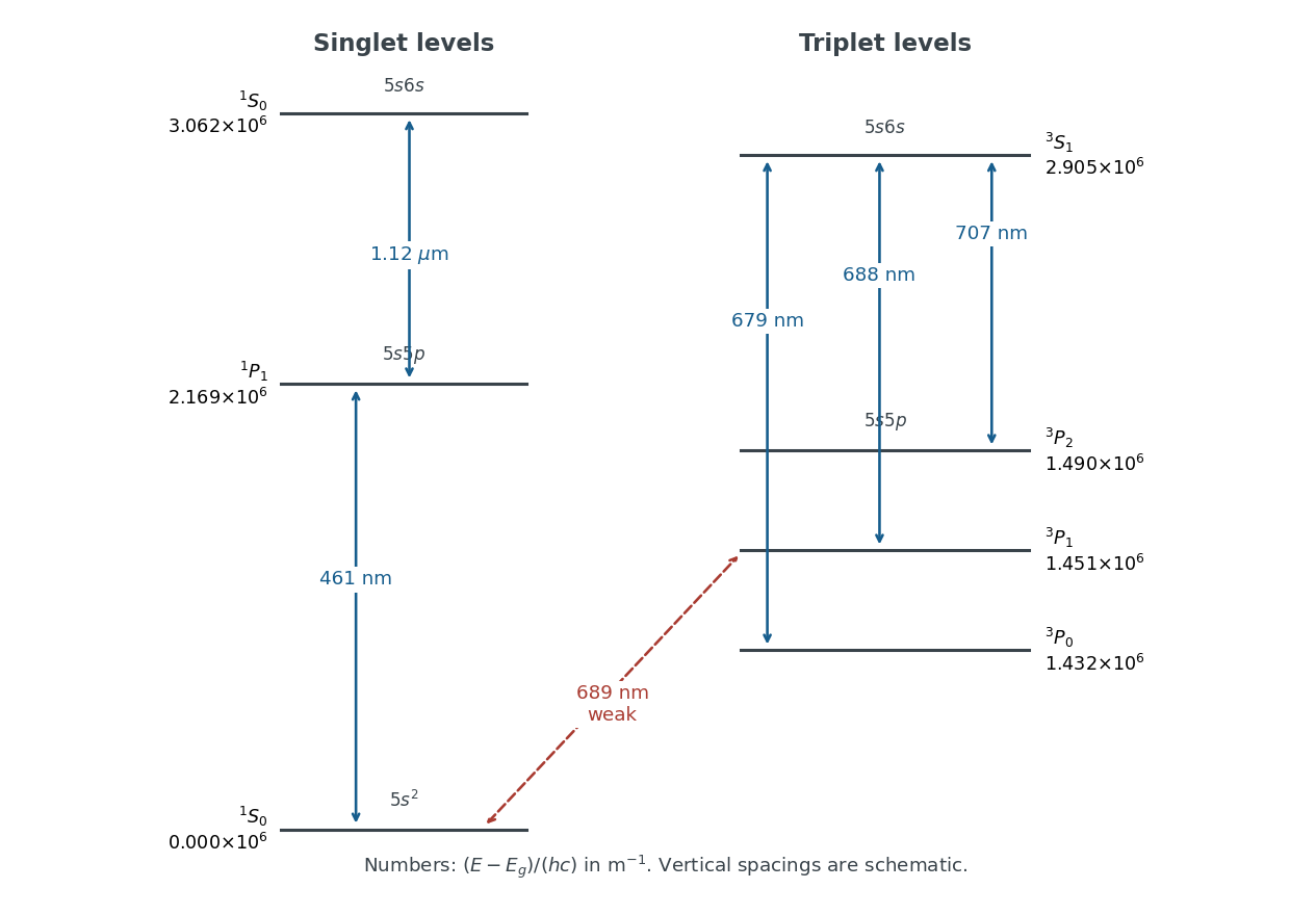
Both $461\mathrm{nm}$ and $1.12\mu \mathrm{m}$ exhibit the normal Zeeman effect. Each connects two singlet state energy levels, with Landé g-factor $g_J=1$ for the $J=1$ energy level and no first-order shift for $J=0$. Their frequency shifts are $0,\pm {\mu }_{B}B/h$. The weak $689\mathrm{nm}$ spectral line also has three components, but $g({}^3{P}_1)=3/2$ gives shifts $0,\pm 3{\mu }_{B}B/(2h)$; a three-component pattern alone does not establish the normal Zeeman effect. The $679\mathrm{nm}$ spectral line likewise has three components with $g({}^3{S}_1)=2$.

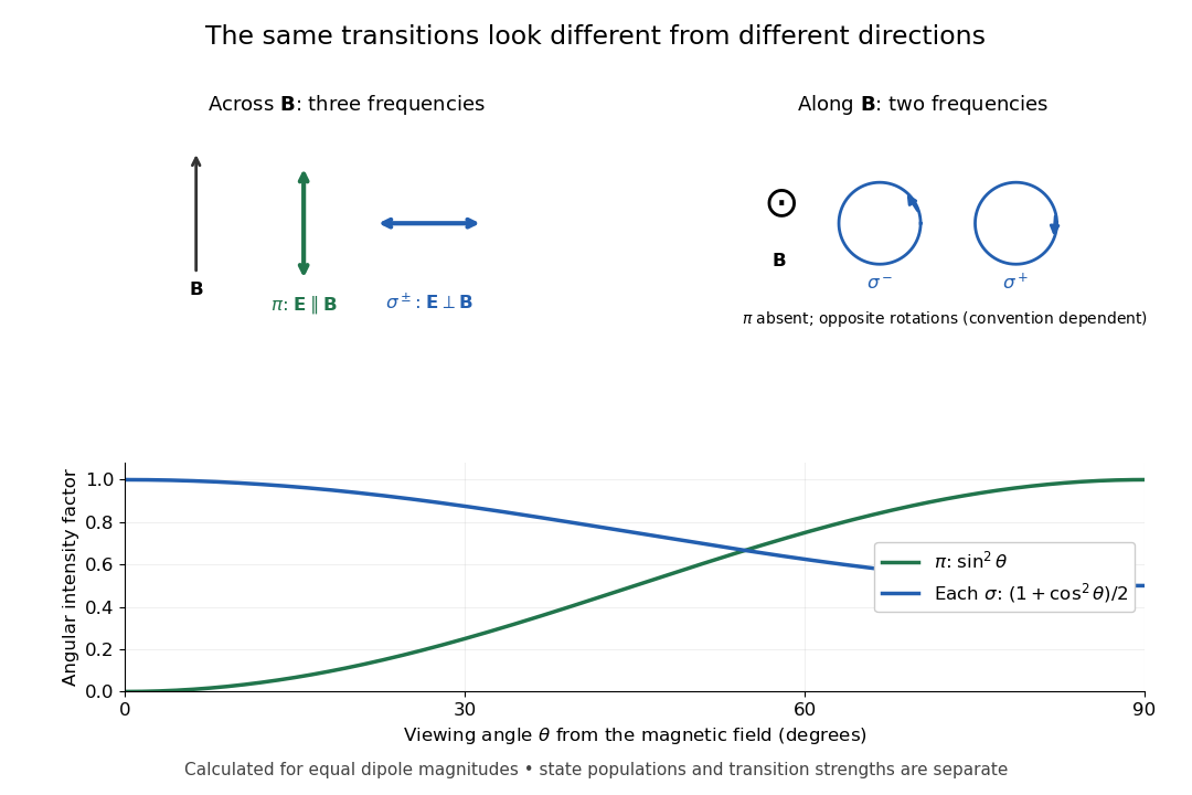
Viewed perpendicular to the magnetic field, the normal Zeeman effect has a $\pi$ component with linear polarization parallel to the magnetic field and two $\sigma$ components polarized perpendicular to it. Along the magnetic field, $\pi$ vanishes and the $\sigma$ pair has opposite circular polarizations. Pieter Zeeman described these geometry-dependent patterns in his lecture.^[ref]

The geometry can be derived from electric dipole radiation. Let the observation unit vector be $\mathbf{n}=(\sin \theta ,0,\cos \theta )$, with $\theta$ measured from the magnetic field. Radiation retains only the transverse part of the oscillating electric dipole moment $\mathbf{d}$:For $\pi$, take $\mathbf{d}\parallel \hat{\mathbf{z}}$; its angular light intensity factor is ${\sin }^2\theta$, so it vanishes on axis. For ${\sigma }^{\pm }$, use normalized complex dipoles $(\hat{\mathbf{x}}\pm i\hat{\mathbf{y}})/\sqrt{2}$. Their angular factors are $(1+{\cos }^2\theta )/2$. Projection gives circles on axis, lines at $\theta =\pi /2$, and generally elliptical polarization between. These factors assume equal dipole magnitudes; actual line light intensities also depend on initial quantum state populations, transition strengths and collection geometry. No absolute handedness name is needed: it depends on the viewing and phase conventions.

A transverse polarizer can separate $\pi$ from $\sigma$ even before the spectral line components are fully resolved. Along the magnetic field, a quarter-wave plate followed by a polarizer converts the two opposite circular polarizations into distinguishable linear settings. This explains why polarization analysis carried information beyond a small increase in line width.