A wavenumber measures how rapidly a wave phase changes with distance. Two conventions coexist: angular wavenumber counts radians per unit length, while ordinary spatial frequency counts cycles per unit length. For a monochromatic wave with wavelength ,Here is the magnitude of the angular wavenumber. The symbol can instead denote a signed one-dimensional angular wavenumber: a factor has wavelength for real . Both conventions have dimensions of inverse length; writing or “cycles per metre” exposes the convention. A quoted value in alone does not resolve the factor of . Spectroscopic wavenumber usually uses the cycles-per-length convention.[ref]
University Physics Volume 1. section 16.2, equations 16.2–16.5: angular convention and sinusoidal wave phase
For a real monochromatic plane wave, fix the conventionThe wavevector supplies both the spatial wave phase slope and the normal to the wavefronts; its dot product with position makes the wave phase constant on parallel planes. The angular frequency is , with the ordinary frequency. Moving a distance along changes the wave phase by . Holding a wave crest's wave phase fixed gives its phase velocity and phase speedIn one dimension the signed phase velocity is . This identifies a moving pattern; it does not identify the motion of the medium's particles or a wave packet's group velocity.
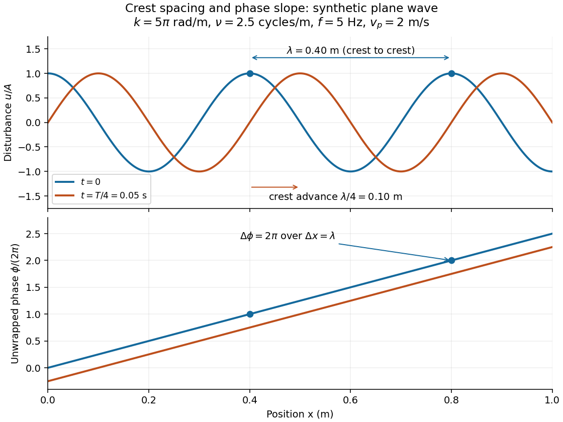
For the synthetic plane wave below, choose and . Then , cycles per metre, , and . The wave crests are apart at one instant; after a quarter oscillation period, each has advanced . The lower panel retains whole turns of wave phase, making its slope visible instead of reducing it modulo .
On a sphere, the integer counts complete zonal oscillations around a latitude circle. Its local Cartesian wavenumber at latitude is for radius . The integer and the dimensional local wavenumber should not be interchanged in a local dispersion relation for Rossby waves.
A complex number used as a wavenumber to encode both spatial oscillation and exponential variation of a wave amplitude. With the convention , a disturbance decaying for increasing has . The sign depends on the convention; thermal diffusion waves provide a concrete example.
A spectroscopic wavenumber commonly means the reciprocal of the vacuum wavelength of electromagnetic radiation, often in . It is an ordinary spatial frequency, so the vacuum angular wavenumber is . Specify vacuum or in-medium wavelength: the same frequency can have different wavelengths in different media. IUPAC's “wavenumber in medium” entry defines the in-medium reciprocal and notes that unqualified spectroscopic usage often means the vacuum reciprocal.[ref]
For example, a vacuum wavelength of corresponds to . Multiplication by gives . Converting centimetres to metres and converting cycles to radians are separate operations.
In spatial sampling of a wave, a detector records a wave at positions separated by pitch . Angular wavenumbers differing by , with integers , give identical samples of a complex Fourier mode:This is spatial aliasing. To distinguish arbitrary sinusoids within a prescribed band, require , equivalently , the Nyquist spatial frequency. Thus for the shortest allowed wavelength. At equality a sine can vanish at every sample, so phase information can be lost. The Nyquist–Shannon sampling theorem states the precise reconstruction conditions for a bandlimited function; a finite scan introduces further limitations.
The synthetic two-tone snapshot iswhere both count cycles per metre. The component wavelengths are and . With , both lie below the Nyquist spatial frequency of cycles per metre. With , the -cycle component aliases to the -cycle component: at every , . The sampled sum is therefore indistinguishable from , although the continuous curves differ between samples. Drawing lines between sample points cannot resolve this ambiguity.
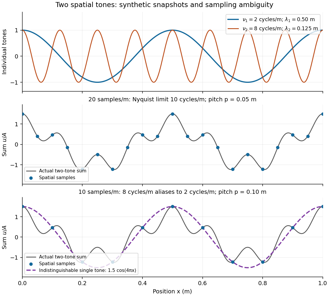
Synthetic two-tone spatial waveform: fine samples distinguish the components, coarse samples hide the shorter wavelength
. Details. The wavelength is the spatial period of a monochromatic wave, measured at a fixed time along the wavevector. For a plane wave with a sinusoid as its profile, it is the distance between consecutive wave crests, or between any consecutive points with the same wave phase modulo :Here uses angular wavenumber, is ordinary frequency, and is phase speed. A distance between arbitrary zero crossings need not be a wavelength: consecutive zeros of a sinusoid are only apart, with opposite slopes. In a standing wave, consecutive nodes of a standing wave are also apart; refers to the constituent travelling waves, even though the nodes of a standing wave do not travel.
Across a stationary interface between stationary linear media, the incident, reflected and transmitted monochromatic waves have the same frequency. The boundary conditions must hold at every time: terms oscillating with different angular frequencies cannot cancel throughout the entire time record. Each medium's dispersion relation then determines its own angular wavenumber and wavelength, soFor electromagnetic radiation in a transparent medium with refractive index , and , where is the vacuum speed of light. A synthetic example with and gives at the same frequency. This conservation argument assumes time-independent linear material response and a stationary interface in the chosen frame. A moving interface can produce a Doppler effect; time-dependent or nonlinear response can change or generate frequencies.[ref]
A broad frequency spectrum generally supplies many component wavelengths, rather than one wavelength for an entire pulse. Even two tones have both their individual wavelengths and a different overall repetition distance: the - and -cycle-per-metre sum in spatial sampling of a wave repeats after , but contains the finer structure. A narrow wave packet can have an approximate carrier wavelength; the wave envelope propagates approximately at group velocity, determined by the slope of the dispersion relation. Substituting that group velocity into generally gives the wrong carrier wavelength. Where the medium varies slowly, local wavelength gives a more useful description.
An acoustic wavelength measurement makes an invisible spatial pattern readable with a ruler. The authored guide Interesting and inexpensive experiments for high school physics by Joe Wolfe places a loudspeaker near a pipe's open end, drives it with an oscillator, and slides a microphone attached to a metre rule through the pipe. An oscilloscope or computer displays the microphone signal. Its oscillation amplitude rises and falls with position; adjacent minima locate pressure nodes of a standing wave a distance apart. A cap gives a pressure antinode at the closed end; an open end has a pressure node just outside it. These are pressure patterns, distinct from displacement patterns. The guide advises wavelengths longer than the pipe diameter, sufficient pipe length to locate both a node and an antinode, and frequency spectrum analysis to distinguish the intended tone from other sounds.[ref]
Interesting and inexpensive experiments for high school physics by Joe Wolfe. pp. 10–11, Standing waves. Reflection and transmission. Speed of sound; apparatus, microphone scan, and pressure-node distinction
The inference follows from superposition of two oppositely directed acoustic plane waves. In an ideal uniform, lossless pipe, taking equal pressure amplitudes and a rigid cap at givesThe time-varying pressure perturbation has local oscillation amplitude . Its zeros are separated by . Unequal incident and reflected amplitudes leave nonzero minima, but their spacing remains in this ideal model. A microphone detects that pressure variation through a changing electrical signal, rather than watching a wave crest move. Record the tone's frequency too, then infer phase speed .
For proposed controls, keep the drive frequency and amplitude fixed during a scan, verify the frequency on the recorded signal, and repeat the scan in both directions. Fit several minimum positions using linear regression to reduce dependence on one pair of positions. Check the ruler scale and use one consistent reference point on the microphone. Compare with the source switched off to locate background measurement noise; use frequency spectrum analysis to check for additional tones, and reduce drive if the trace ceases to resemble a sinusoid. Record air temperature and avoid strong air motion. These are suggested controls, not additional procedures or observations attributed to the guide.
The pipe must support approximately plane waves over the measured region: transverse structure at shorter wavelengths, the microphone's finite size, and disturbance by the ruler can compromise the interpretation. Weak reflection gives shallow minima, while damping and other reflections can shift the extrema of the simple two-wave model. Measure interior spacings rather than assuming the first minimum is exactly at the pipe lip. A short scan may not include enough minima to estimate reliably, and drift during sequential scanning can imitate spatial variation.
For an explicitly hypothetical calculation, and give , , and . No such measurements are claimed here. If independent small measurement errors in and fitted have standard deviations and , first-order error propagation gives . A systematic scale error or changing air conditions requires separate assessment.
An oscilloscope displays an electrical signal versus time. In an acoustic wavelength measurement, the microphone trace supplies the tone's frequency and oscillation amplitude as the detector changes position.
A connection that couples a measured electric potential difference into an oscilloscope. Its electrical resistance and capacitance contribute to instrument loading.
Propagation of uncertainty estimates how measurement errors in inputs affect a calculated result. For small input errors with covariance matrix , linearizing a differentiable function gives the displayed approximation for its variance. For independent errors in a product , the squared relative standard deviations add. Correlated errors need the covariance terms; systematic offsets require separate assessment.
If measured radiative flux is and with known , first-order uncertainty propagation gives the displayed result. Independent measurements have zero covariance; strict error bounds combine differently. Even a small fractional background contribution can matter if its relative uncertainty is large. Inferring the covariance or an unknown calibration factor from precision percentages alone is unjustified.
For , the sensitivity coefficients are and . The first-order uncertainty propagation law gives the displayed variance; independent inputs remove the covariance term. Subtracting a known constant does not change absolute uncertainty, but can greatly change relative uncertainty when the resulting value is small. The result is a standard uncertainty estimate, not automatically a worst-case error bound or a confidence interval.
For with reactance , linear differentiation gives . Independent standard uncertainties give the title formula; correlated inputs add . Hard error bounds instead add absolute linear contributions. The meaning of an error bar is an additional measurement assumption, not a consequence of the impedance formula.
For air approximated by index one, , so . Taking the variance gives the displayed first-order error formula, with angles and their errors in radians. Independence removes the covariance term; hard error bounds require a different combination rule. Common angular-zero errors can produce covariance and should not automatically be added in quadrature.
For axial moment of inertia , linear sensitivity to mass and outer/inner radius is . Independent standard uncertainties give . Correlated measurements instead require the full covariance quadratic form. For deterministic bounds, add the absolute linear contributions rather than their squares.
For with independent standard uncertainties, linear propagation gives . Angular uncertainty must be in radians when using this derivative. Covariance adds cross terms for correlated inputs. Strict error bounds instead add absolute first-order contributions; they do not justify Gaussian significance tests.
For positive measured inputs and , logarithmic differentiation gives . Applying propagation of uncertainty yields the displayed covariance formula. For independent input errors it reduces to . If the input uncertainties are strict bounds rather than standard deviations, a first-order conservative bound is . These are different statistical interpretations; a product formula alone does not choose between them.
For the same massless spring obeying Hooke's law, the frequency is . The displayed mass ratio follows. For small independent frequency errors with common fractional standard uncertainty , monomial uncertainty propagation gives . If instead describes individual measurements and each sample mean uses independent trials, its standard error is smaller by , giving . Four times as many trials halve this statistical uncertainty; a common calibration error needs its covariance included.
For simple pendulum oscillation period in the small-angle approximation, . If the length measurement and identically precise timing measurements have independent errors, the timing sample mean has standard error . Propagation of uncertainty gives the title formula. A target fractional standard uncertainty requires , rounded upward to an integer. No amount of repeated timing can beat the floor without improving the length measurement; correlated errors or a timing systematic error require a different model.
For a locally oscillatory wave written , the local wavevector is , where is the spatial gradient. The local wavelength measures local wave phase spacing normal to the wavefront. Interpreting it as a crest separation requires the amplitude and local wavevector to vary little over one wavelength, as in the WKB approximation. Along a unit direction the corresponding local repeat distance is , if that dot product is nonzero; oblique sampling measures this projected spacing.
A real snapshot alone does not uniquely specify and : their meaning requires a chosen oscillatory component or physical approximation. Strong interference, zeros of amplitude, and rapidly changing media can defeat a single-carrier description. If , the local reciprocal formula gives no finite wavelength; it does not establish an exact global spatial period.
Articles by others on the same topic



Wavenumber is a measure of the number of wavelengths per unit distance and is used in various fields such as physics, chemistry, and optics. It is defined as the reciprocal of the wavelength and is usually expressed in units of reciprocal length, such as inverse meters (m⁻¹).