Compute all three components of the Cartesian curl explicitly:Thus throughout . There are no excluded singular points in this polynomial field.
The field is continuously differentiable on all of , a simply connected domain. Its vanishing curl therefore implies a global potential of a conservative vector field, so is an exact differential. This global domain condition matters: curl-free fields on domains with holes need not have single-valued potentials.
Integrating gives . Matching forces , so ; matching then forces . ConsequentlyThe additive constant does not affect the field or any endpoint difference.
On the specified parametrized curve, and . Substitution into the field gives . HenceThe line integral is thereforeBoth the field and the tangent vector must be evaluated along the curve; integrating one field component alone would miss two contributions.
Interpret the axis-directed route as successive coordinate-axis-parallel segmentsOn the first segment, , so the field vanishes. On the second, , so it again vanishes. On the last, , and only is nonzero, giving . ThusThe second and third segments are parallel to the corresponding global axes; they do not return to the global - or -axis before reaching the endpoint.
Both paths start at and end at . The potential values are and , soThis is the fundamental theorem for line integrals: an exact one-form integrates to the difference of its single-valued potential at the endpoints. The agreement is guaranteed for every piecewise smooth connecting path, rather than being an accident of these two examples. In particular the integral around a closed path assembled from one route and the reverse of the other is zero.
Stokes theorem stateswith boundary orientation induced by the chosen surface normal and with sufficient smoothness of the field and surface. Choose the outward normal on the upper unit hemisphere; its equatorial boundary runs counterclockwise as viewed from .
For the stated field, the curl isOn the unit sphere, the outward normal is . In spherical coordinates, the surface integral over the upper hemisphere isFor the boundary calculation, parametrize , with . Then andThus both sides equal . Reversing the hemisphere orientation reverses both signs. The hemisphere's flux calculation can also be read as the projected area of its equatorial unit disk.
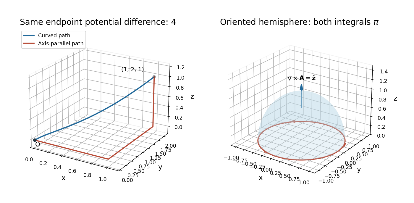
Two equal-endpoint paths and the oriented hemisphere used in Stokes' theorem
. Details. 
Articles by others on the same topic
There are currently no matching articles.