Source paper: Oxford source archive, member
2015/CP4_June_2015.pdf. The cover dates this ordinary paper to 11 June 2015. All four Section B options and all inline Roman subparts are treated.For a continuously differentiable vector field on a volume with piecewise smooth boundary , the divergence theorem stateswhere is the outward unit normal. For the polynomial field here,Therefore the outward flux through the unit cube isAs a direct boundary check, the face contributes , the face contributes , and the face contributes . All three opposite faces contribute zero, reproducing the result and fixing the orientation sign.
The Maclaurin series cancels the numerator's linear term, leavingThus . The same expansion applies for positive and negative , so this is a two-sided limit.
Combine the terms before taking their limit:Using the exponential function Maclaurin series, the numerator is and the denominator is . ConsequentlyThe cancellation removes the two individual singularities. Subtracting their separate divergent limits would not determine the finite answer.
Write . Multiplying by the cosine Maclaurin series and comparing with the sine series givesCoefficient comparison yields , and . HenceSubstitute into . Keeping one extra order to make the term-counting explicit,Counting the constant term, the first three nonzero terms are . If the phrase is taken to mean the first three nonconstant terms, they are ; the displayed expansion supplies both conventions. The cubic coefficient is , combining the cubic term in with the cubic exponential term.
For , the radial vector field has components . The product rule givesThus for ,When , and the ordinary divergence is zero at every nonzero radius. However, the field is singular at the origin. Its outward flux through a radius- sphere is , so one cannot apply the smooth-field divergence theorem across the origin and conclude that this flux vanishes.
In the language of distributions, the complete distributional divergence identity is . Here is the three-dimensional Dirac delta function. Without that generalized interpretation, the correct statement is simply zero divergence away from the origin and undefined ordinary divergence at the singular point. Removing a small ball around the origin restores the ordinary theorem: the inner boundary has inward radial orientation and cancels the outer flux.
For phase , a constant-phase point moves at the phase velocity . A narrow-band wave packet has envelope speed given by the local group velocity on its dispersion relation.
Since ,Use the in-medium wavelength , so . The velocity relation becomesThe stated increase of phase velocity with wavelength means . Therefore . The inequality alone does not provide their numerical values or guarantee a positive group speed for an arbitrary dispersion law; it fixes their ordering. For ordinary transparent glass in its normal-dispersion band, both are positive and the group speed is the smaller one.
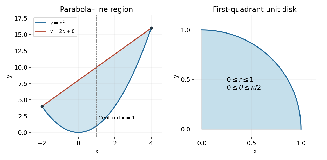
The boundaries intersect where , giving and . Between these values, the straight line lies above the parabola. ThereforeEvaluation givesA useful independent check uses the region's symmetry about : its vertical width is . Its area is , and its centroid has coordinate one, so its first moment is again .
The integration limits describe the first-quadrant quarter of the unit disk: , , . Its circular boundary and the axes are shown in the right-hand panel below; the left panel gives the bounded region used in the preceding calculation.
Use polar coordinates , with and . The Jacobian determinant gives , soThus . Including the radial Jacobian is essential; the exponential becomes radial, but the area element does not remain .
Take the constant speed parameter , so and are independent characteristic coordinates. The chain rule givesApplying these operators twice to a twice differentiable function yieldsConsequently the wave equation reduces to . Integrate first with respect to , obtaining , and then with respect to , allowing a separate integration function of . The general local solution iswith arbitrary sufficiently differentiable functions and . For , the first profile travels towards negative and the second towards positive . Substitution directly checks the equation. Initial or boundary conditions select the two profiles; none are specified here. This is D'Alembert's formula in characteristic form.
The first partial derivatives areIf , then , so no stationary point is lost by excluding those values. The remaining condition forces , and then givesThere are infinitely many such points. On every tangent branch , the function has derivative and goes from to . The intermediate value theorem and strict monotonicity therefore give exactly one root on every branch. The central root is , and oddness pairs the other roots at opposite signs.
For increments and , the second-order multivariable Taylor expansion isAt a stationary point , and . Direct differentiation givesThus, since this particular function is analytic, the expansion can be writtenThere are no linear terms because the gradient vanishes, and no mixed quadratic term because the mixed derivative vanishes on the axis.
At a stationary point of a twice continuously differentiable function, write the Hessian matrix as and its determinant as . The quadratic term in the Taylor expansion determines the local nature whenever is nonsingular.
If , its two eigenvalues have the same sign. With the quadratic form is positive definite, giving a strict local minimum; with it is negative definite, giving a strict local maximum. If , the eigenvalues have opposite signs and the point is a saddle, with nearby increasing and decreasing directions. ThusIf , the test is inconclusive. For example, , and all have zero gradient and zero Hessian matrix at the origin, yet give a minimum, a maximum and a saddle respectively. One must inspect higher-order terms or use another argument in such a case.
For every stationary point found above, and hence . The Hessian matrix is diagonal, with entries and , soThe entries always have the same sign. ThereforeThe root on tangent branch has cosine sign . Thus even-numbered branches supply maxima and odd-numbered branches minima, symmetrically paired about the origin. There are no saddle points among these nondegenerate stationary points. The origin is a maximum with , and is in fact the global maximum since and .
For , the first derivatives are and . Both vanish at the origin. The local expansion isThere are no constant, linear or quadratic terms, so every second derivative vanishes at the origin and the Hessian determinant is zero. The second-order test therefore cannot classify the point.
The cubic term does determine the behaviour: along , has the sign of . Every neighbourhood contains values above and below , so it is neither a maximum nor a minimum. It is a nonisolated stationary point with nearby values of both signs. Indeed the whole line is stationary, so this is not an isolated nondegenerate quadratic saddle.
Let be displacements from equilibrium, with positive directions chosen alike. Hooke's law and Newton's second law giveFor a normal mode , the determinant condition isSolving the quadratic for givesThe angular frequencies are the positive square roots. Positive masses and spring constants make the stiffness quadratic form positive definite, ensuring both squared frequencies are positive. Distinct spring constants do not require equal masses or any symmetry approximation.
Put and . The mass-normalized stiffness matrix isIts symmetric eigenvector has eigenvalue , while its antisymmetric eigenvector has eigenvalue . ThusThe symmetric frequency does not depend on the middle spring constant because that spring has no extension in an in-phase normal mode. The antisymmetric motion stretches the middle spring and has the higher frequency for .
With the same positive displacement convention for both masses, the first eigenvector equation is . At the symmetric frequency it reduces to , while at the antisymmetric frequency it becomes . HenceIn both normal modes the displacement magnitudes are equal. For the first, the masses move in phase and their separation stays unchanged; for the second they move in opposite phase, alternately approaching and separating. A negative signed amplitude ratio records a phase difference of , not a negative displacement magnitude. The left panel of the later figure plots these signed normal mode shapes with the fixed wall values included.
Both masses in the source's absorber diagram are free: there is no additional spring attaching to a wall. Let their displacements be and . The equations areFor a periodic particular response , , the amplitude equations are and . Their solution isAt , and : the spring force on the larger mass cancels the applied force at every instant. This is antiresonance, a frequency-selective cancellation, rather than dissipation of energy.
There is a nearby undamped resonance at . For it lies close to the cancellation setting. More quantitatively, write . ThenFor , the amplitude relative to the unconnected mass's amplitude is approximately . A light absorber therefore needs very accurate tuning and loses suppression when the driving frequency changes. Its own travel can also become large, limiting linearity and available stroke.
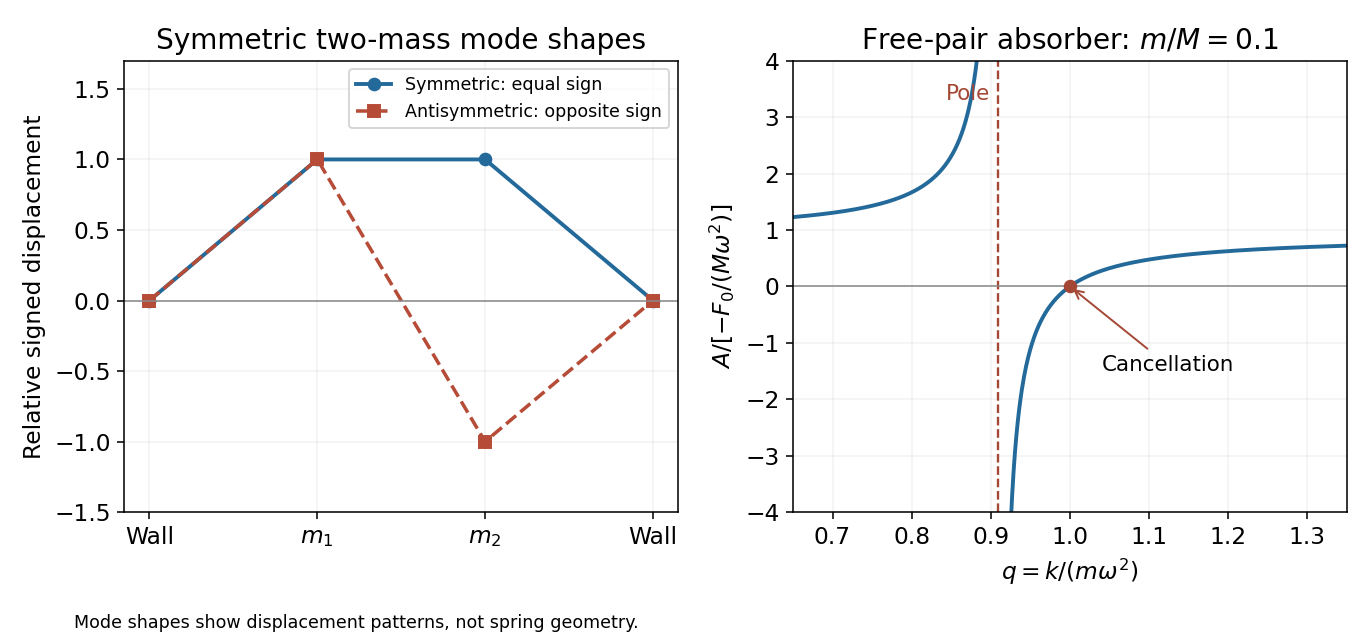
Without damping, resonance growth and persistent free oscillations remain; special initial conditions select the displayed periodic particular response. The free pair also has rigid-translation motion. These limitations prevent interpreting the cancellation as broadband damping or as a unique attracting late-time state.
For an equilibrium string segment of length , the mass is . Under the small-slope approximation, the transverse tension component at an endpoint is . The difference between its two endpoint contributions is .
Newton's second law in the transverse direction gives . Cancelling the segment length producesThis wave equation assumes a uniform string, small slopes, negligible gravity and negligible bending stiffness. Longitudinal changes in tension and the difference between actual and equilibrium segment length contribute only beyond the linear approximation used here.
The instantaneous energy flux towards positive is the rate at which the string on the left does work on the string on the right. To first order its transverse force is , soFor a right-travelling sinusoidal wave , and . ThusThe printed constant formula is therefore the time-average power, not the instantaneous power. The latter oscillates between zero and twice its average. A left-travelling wave carries negative signed flux through the same positively oriented section; its transported power magnitude has the same average formula with positive .
Place the massless junction at , with common tension on both sides. Using a common time factor , write the left-hand wave as and the right-hand wave as . A stationary junction does not change the frequency, while .
displacement continuity requires . Transverse force balance on a massless junction requires equal tension-weighted slopes, giving . Hence the signed displacement coefficients areHere , so and . The negative reflected coefficient signifies inversion. If “reflection and transmission coefficients” instead denotes power fractions, their values are and , as derived separately below; power and displacement coefficients must not be conflated.
The transmitted and incident waves have the same angular frequency and tension, but the transmitted wavenumber is twice as large. The time-average string-power formula therefore givesThe extra factor is essential. Squaring the displacement transmission coefficient alone would give , which is not the transmitted power fraction in strings with different linear mass densities.
The reflected wave remains on the incident string, so its wavenumber magnitude is still . Its outward power magnitude isThus , verifying energy conservation. With signed positive- fluxes, and the same statement is . The minus sign of the reflected displacement is a phase reversal, whereas the minus sign of its flux records travel in the opposite direction; these are different uses of a sign.
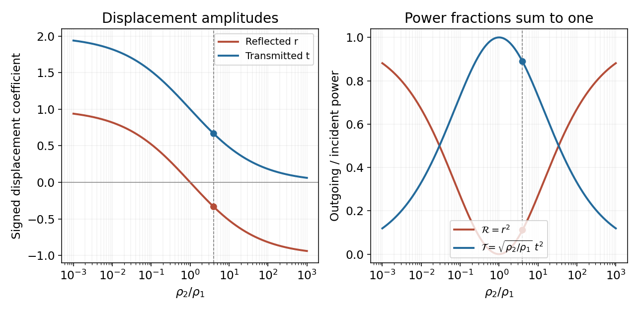


For equal linear mass densities and common tension, . The junction relations then giveThere is no mechanical-impedance discontinuity, so no reflected wave is needed to satisfy displacement and force continuity. The transmitted displacement is in phase with the incident wave and has the same amplitude; all incident power crosses the junction.
If , then and the wave meets a much larger string impedance. The displacement and power coefficients approachThe junction behaves approximately as a fixed end. The reflected displacement reverses sign, corresponding to a phase shift of ; the small transmitted displacement is not inverted. For a large but finite density ratio, and the transmitted power fraction is about , tending to zero rather than vanishing identically at every finite ratio.
If , then and the junction behaves approximately as a free end for the incident string. The limits areThe reflected displacement is not inverted, and at the junction it adds in phase to the incident displacement, producing nearly twice its amplitude. The transmitted displacement is also in phase. A transmission amplitude near two does not create power: the lighter string has much smaller impedance, and . These are limiting statements for positive densities, not an ordinary propagating-wave model for an exactly massless second string.
Compute all three components of the Cartesian curl explicitly:Thus throughout . There are no excluded singular points in this polynomial field.
The field is continuously differentiable on all of , a simply connected domain. Its vanishing curl therefore implies a global potential of a conservative vector field, so is an exact differential. This global domain condition matters: curl-free fields on domains with holes need not have single-valued potentials.
Integrating gives . Matching forces , so ; matching then forces . ConsequentlyThe additive constant does not affect the field or any endpoint difference.
On the specified parametrized curve, and . Substitution into the field gives . HenceThe line integral is thereforeBoth the field and the tangent vector must be evaluated along the curve; integrating one field component alone would miss two contributions.
Interpret the axis-directed route as successive coordinate-axis-parallel segmentsOn the first segment, , so the field vanishes. On the second, , so it again vanishes. On the last, , and only is nonzero, giving . ThusThe second and third segments are parallel to the corresponding global axes; they do not return to the global - or -axis before reaching the endpoint.
Both paths start at and end at . The potential values are and , soThis is the fundamental theorem for line integrals: an exact one-form integrates to the difference of its single-valued potential at the endpoints. The agreement is guaranteed for every piecewise smooth connecting path, rather than being an accident of these two examples. In particular the integral around a closed path assembled from one route and the reverse of the other is zero.
Stokes theorem stateswith boundary orientation induced by the chosen surface normal and with sufficient smoothness of the field and surface. Choose the outward normal on the upper unit hemisphere; its equatorial boundary runs counterclockwise as viewed from .
For the stated field, the curl isOn the unit sphere, the outward normal is . In spherical coordinates, the surface integral over the upper hemisphere isFor the boundary calculation, parametrize , with . Then andThus both sides equal . Reversing the hemisphere orientation reverses both signs. The hemisphere's flux calculation can also be read as the projected area of its equatorial unit disk.
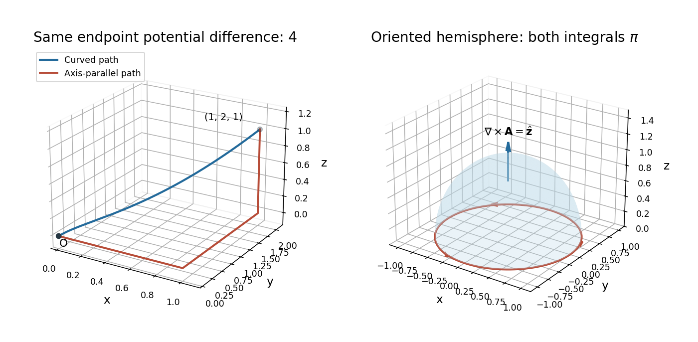
Two equal-endpoint paths and the oriented hemisphere used in Stokes' theorem
. Details. 
Articles by others on the same topic
There are currently no matching articles.