Take small incoming sections and outgoing sections after straightening the stable manifold and unstable manifold of the origin. Its eigenvalues are , so the leading local passage satisfies , . The exit time and transverse exit coordinate areThus the local passage contracts strongly as , while its duration diverges. Smooth global reinjection from the right outgoing section to the upper incoming section has leading transverse coordinate ; the corresponding left-to-lower return has . Choose the parameters as these signed splitting coordinates and absorb into .
After scaling the incoming-section labels to , the leading Poincaré return map isThe second coordinate records which outgoing branch was used, not an independent continuous amplitude. A smooth planar flow preserves the orientation of a transverse-section return. For the right-to-upper pair of sections, the ordered pair consisting of the flow direction and the positive section tangent has the same orientation at both ends; the same is true for the left-to-lower pair. Hence for these sign conventions and a nondegenerate global return.
For general nonlinear , this is an asymptotic return model, with smooth parameter corrections and higher-order local-passage corrections. The hypotheses do not imply an exact power-law map in the original coordinates. Interpreting the printed parameters themselves as linear splitting coordinates also requires a nondegenerate two-parameter unfolding: the two splitting derivatives must be nonzero. For example, composing a generic right-loop splitting with preserves the stated loop at but does not give the printed signed offset. The subsequent region diagram uses the standard generic splitting-coordinate interpretation. Nor is a normal return point: it lies on the stable manifold, whose trajectory takes infinite time to reach the saddle equilibrium. This explains how the map describes nearby recurrent trajectories without extending a finite-time return across the singular separatrix.
We count periodic orbits whose trajectories remain near the two specified homoclinic orbits; the local hypotheses impose no bound on unrelated distant cycles. Choose the return domain small enough that and are less than one. Each admissible return branch is then a contraction mapping.
A right-lobe periodic orbit is a fixed point with and . For small amplitudes it exists exactly when , and . Similarly, a left-lobe periodic orbit has , , , and exists for . Their Floquet multipliers tend to zero, so both are attracting.
A period-two orbit of the section map corresponds to one flow periodic orbit traversing both lobes. Write its states as and . Its positive amplitudes satisfyThe two-step derivative is , again tending to zero. The asymmetric planar gluing return map therefore gives at most one such attracting two-lobe cycle in the small domain. Its boundaries are obtained by setting one amplitude to zero:For the original flow these are leading equations, with corrections or . On , the negative unstable branch makes both excursions before returning to the positive stable branch; on the positive unstable branch returns to the negative stable branch. Each is a compound homoclinic orbit, with one extra passage near the saddle equilibrium. They are distinct from the primary loop curves and .
The six open regions and their local cycles are:
| Region | Attracting flow cycles |
|---|---|
| Right and left single-lobe cycles | |
| Right single-lobe cycle only | |
| Right single-lobe cycle and two-lobe cycle | |
| Left single-lobe cycle only | |
| Left single-lobe cycle and two-lobe cycle | |
| Two-lobe cycle only |
There is no additional small alternating cycle when both parameters are negative. Indeed the two positive-amplitude equations would imply and , giving , impossible for sufficiently small positive . On each mixed-sign quadrant the contraction equations give the two-lobe cycle precisely on the side of the compound curve toward the positive quadrant.
On , there is the primary right homoclinic orbit, together with a left cycle if or a two-lobe cycle if . On the analogous statement holds with left and right interchanged. On there is a compound homoclinic orbit and the right single-lobe cycle; on there is a compound homoclinic orbit and the left single-lobe cycle. At the two primary loops meet at the same saddle equilibrium. The approach to each homoclinic orbit has a diverging period; it is not a saddle-node collision of two finite-period cycles.
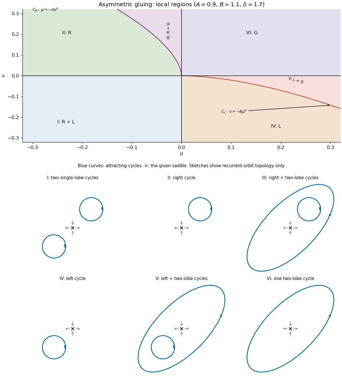
Parameter regions and schematic phase portraits for asymmetric planar gluing
. Details. 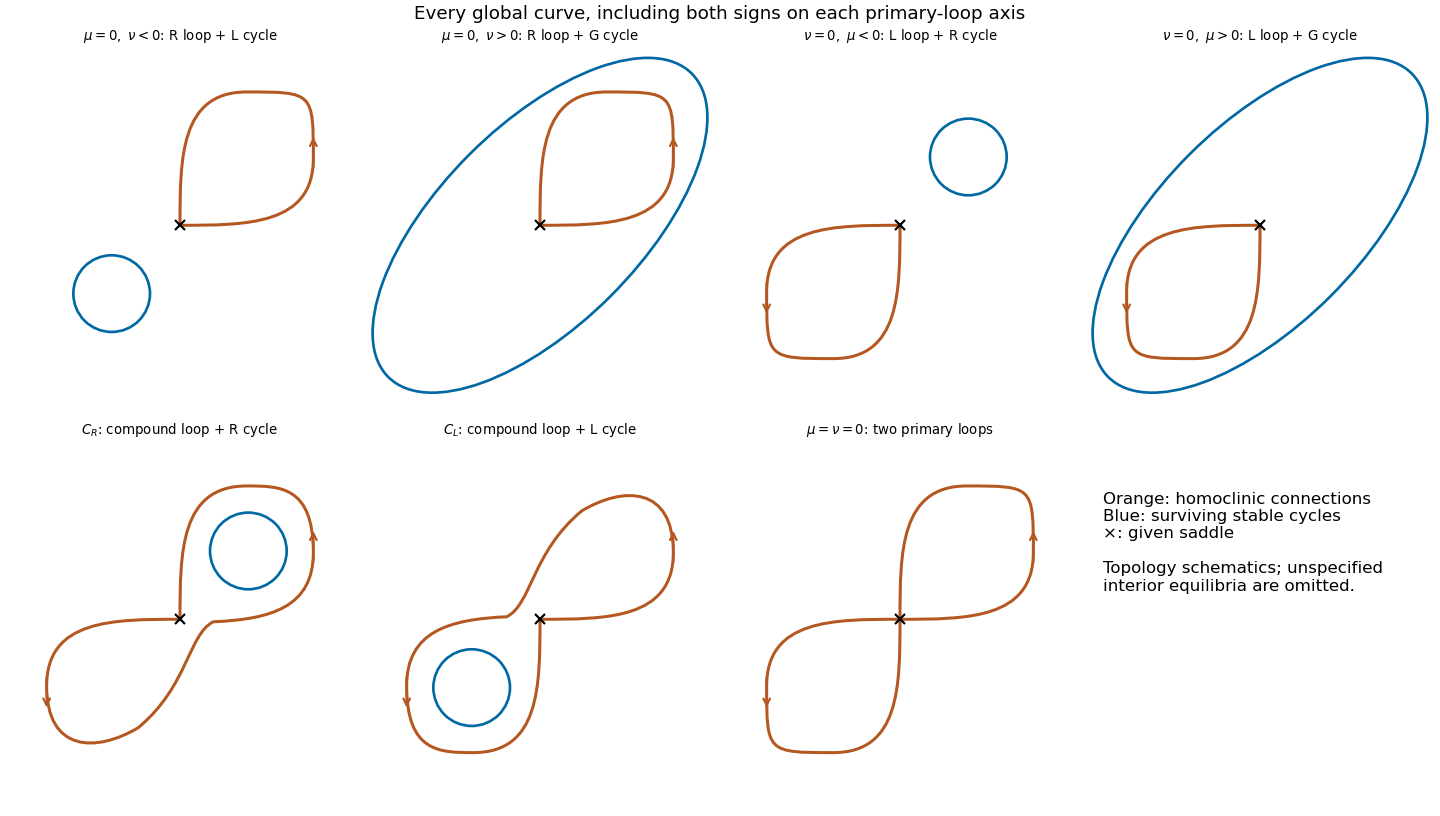


With reflection symmetry, choose and . The two primary homoclinic orbit curves are then encountered simultaneously at . For the return has two attracting single-lobe cycles; for it has one attracting two-lobe cycle. This is the symmetric homoclinic gluing bifurcation: two cycles meet the two saddle loops and are replaced by a cycle traversing both lobes. Since , the saddle equilibrium contracts strongly enough for the nearby cycles to be stable.
One can also use the signed gluing-map reduction . In the symmetric return map it gives . A negative fixed point lifts to two reflection-related flow cycles; a positive fixed point lifts to one period-two orbit of the two-sheet section map, hence one two-lobe flow cycle. This distinction prevents counting the two section intersections as two different flow cycles.
Without reflection symmetry the two splitting parameters are independent. The primary loops occur separately, and the two compound curves bound small coexistence wedges where a single-lobe and a two-lobe cycle are both stable. Thus the six-region picture is the generic two-parameter unfolding of the symmetric gluing event. The simultaneous encounter of both primary loops is codimension two for a general planar flow but codimension one in the reflection-symmetric family. The contraction argument applies to the small return domain; it makes no assertion that a globally arbitrary system has only these cycles everywhere.
Articles by others on the same topic
There are currently no matching articles.