At both points, and , so both components of the vector field vanish. Thus both points are equilibrium points for every parameter value. These are regular points of the spherical coordinates chart: the coordinate singularity at the pole plays no role in their linearization.
Use local coordinates , at . The Jacobian matrix, its trace and its determinant areConsequently is attracting when , repelling when , and a saddle equilibrium when . A transition between a node and a focus at changes the linear geometry but is not a bifurcation of the local topological phase portrait.
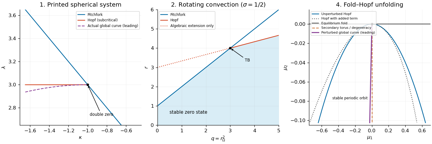
The stationary bifurcation curve is . To identify it, write , . At a non-equatorial equilibrium point, eliminating givesNear , if , these yield and . The two branches are related by the local reflection . Their determinants are , so they are saddle equilibria. This is a pitchfork bifurcation; on the portion with the saddle branches lie on the side where is stable, giving a subcritical pitchfork bifurcation.
A Hopf bifurcation requires , henceThe oscillation frequency is . At the intersection , but : there is a double zero eigenvalue with one eigenvector. The map from to has nonzero Jacobian determinant, so two independent parameter conditions produce this codimension-two bifurcation. Reflection removes quadratic terms; the appropriate initial comparison is with a reflection-symmetric cubic double-zero normal form, subject to the cubic degeneracy checked below.
For completeness, the printed vector field has a subcritical, rather than supercritical, Hopf bifurcation. In the mechanical coordinates , , at its cubic acceleration has coefficient and coefficient . For a small harmonic oscillation, the averaged cubic change of is , whereThus a small unstable periodic orbit lies on the attracting side of the Hopf bifurcation. This calculation matters when comparing the original equations with the later assumed normal form.
The cubic Taylor expansion at the double-zero point isThere are no quadratic or quartic terms because the local vector field is odd under . Set , , and use . The linear transformation is invertible, and the positive time rescaling preserves orbit orientation. With primes denoting , the result isThis supplies the requested cubic functions, with a remainder stronger than .
There is an important normal form check. Setting , straightens the first equation, and differentiating givesIn particular the nilpotent cubic damping invariant is . A nonsingular cubic near-identity transformation and rescaling cannot change this vanishing invariant into the nonzero coefficient in the supplied later normal form. The conclusions for that assumed system are therefore given separately from the independently derived conclusions for the printed original equations.
First analyze the supplied normal form as a dynamical system in its own right. Its equilibrium points are and, for , . At , the trace is and the determinant is . At , the determinant is , so both are saddle equilibria. Thus is the pitchfork bifurcation curve, and is the Hopf bifurcation curve. With the allowed supercritical Hopf bifurcation, an attracting limit cycle is born on around the repelling origin.
The Hamiltonian obeys . Set , , , , and . The limiting Hamiltonian system has two oppositely directed heteroclinic orbits with for . The Melnikov energy-balance method givesIts unique simple zero gives a heteroclinic cycle curveThe two connections occur on the same curve because reflection interchanges them. The attracting limit cycle grows toward this heteroclinic cycle, then disappears. In the small unfolding neighborhood there is one such connection curve, rather than two independently split curves. There are no nearby homoclinic orbits replacing it: the two equal-height outer saddles are the relevant separatrix endpoints.
This calculation transfers to the original equations only if the asserted reduction is valid. The cubic calculation in part (c) shows it is not valid for the printed coefficients. Nevertheless, the claim of a single nearby global bifurcation curve for the original equations can be proved independently. Put , , , , and . Eliminating using producesThe order- correction is reversible and has no first-order separatrix energy imbalance. On the limiting positive connection, and . The first dissipative balance isAgain the zero is simple, and reflection makes the two heteroclinic orbits simultaneous. Hence the actual original equations have the unique local connection curveThe unstable limit cycle on the subcritical Hopf bifurcation side reaches this curve. Thus the original system still has one nearby global connection curve, but its tangency and cycle stability differ from those of the supplied assumed cubic normal form. These statements concern connections contained in the shrinking neighborhood of ; they do not exclude unrelated distant global bifurcations elsewhere on the sphere.
For the supplied normal form, the four local topological phase portraits are as follows. When , only the origin is present and it is a saddle equilibrium. When , the origin is attracting, between the two outer saddle equilibria; inward-facing separatrices enter its basin. When and , the origin is repelling and a stable limit cycle surrounds it, inside the separatrix boundary formed by the outer saddle equilibria. Finally, when , the origin remains repelling but the local limit cycle has disappeared, and trajectories leave the central region through the opened separatrix channels. Whether the origin is a node or a focus within one of these regions does not change this orbit topology.
On the connection curve, the two outer saddle equilibria are joined in both directions; the period of the disappearing limit cycle diverges. This is a heteroclinic cycle, not a pair of saddle homoclinic orbits. The sketches below show the four open regions of the supplied system; they are not presented as phase portraits of the inequivalent printed spherical equations.
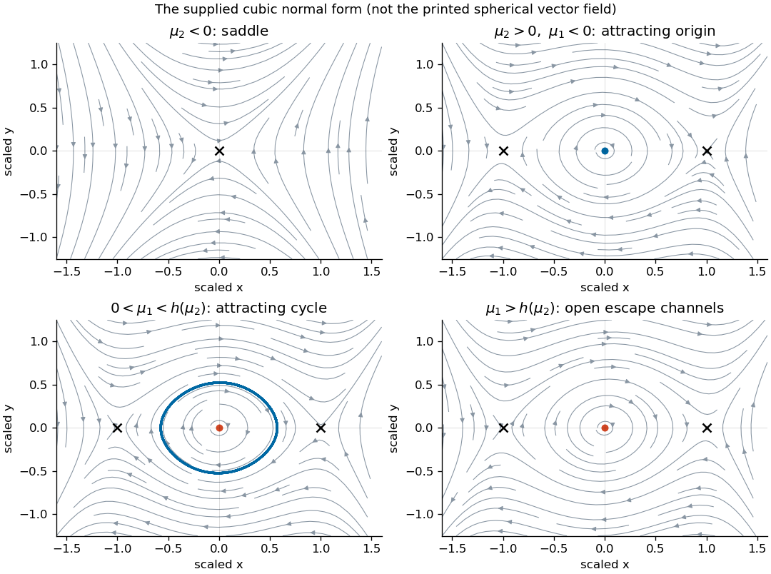
Four phase portraits of the supplied reflection-symmetric cubic normal form
. Details. Use the Galerkin method: substitute the retained trigonometric modes and project onto them with the inner product over the rectangle. Each mode satisfies the printed boundary conditions. Write , , and abbreviate the four mode prefactors by , , and . The Jacobian determinant in the advection terms is .
The stream function is a single Laplacian eigenfunction, so and exactly. For the temperature modes, direct multiplication givesFor the transverse-velocity modes, the retained products areFor example, and supply the signs of the two retained and couplings. The third harmonics are orthogonal to the retained modes and are discarded by this Galerkin method; they are not claimed to vanish in the full partial differential equations.
Before changing time, the five coefficient equations areDividing by gives the stated five-mode rotating-convection truncation, withThe squared rotation parameter is . The printed is proportional to rotation rate, so it is a square-root-type rotation parameter rather than the more usual Taylor number proportional to squared rotation rate; the algebra uses the coefficient as printed. At zero rotation the physical transverse velocity modes vanish; the normalized equations can still be understood through their continuous zero-rotation limit.
Let and . The eigenvalues at the conductive equilibrium point are and , both negative since and . The coupled Jacobian matrix has characteristic polynomialwhereA simple zero eigenvalue occurs on . The reflection , with fixed, makes its generic steady-state bifurcation a pitchfork bifurcation.
For a nonzero imaginary pair, substitute into : the real and imaginary parts require and . HenceWith , this Hopf bifurcation curve is present only for . At its intersection with the pitchfork bifurcation curve,and . The zero eigenvalue has geometric multiplicity one: its eigenvector has , . Thus this is a reflection-symmetric Bogdanov–Takens bifurcation, rather than two independent zero modes.
The Routh-Hurwitz stability criterion gives the stable trivial state below for and below for . The rest of the line , beyond , is a stationary bifurcation of an already unstable trivial state. Likewise the extension of below is only an algebraic line, since its putative frequency is not real. The middle panel of the bifurcation diagram in part 1(b) distinguishes the actual curves from this extension.
To determine the nonlinear pitchfork bifurcation, solve the four slaved steady equations exactly. SetThe nonzero equilibrium points satisfyThusIf , the coefficient of is positive for every physical : there is no change of pitchfork direction at a nonnegative rotation parameter. If , the change occurs atBelow the nonzero branch lies on ; above it initially lies on . At , , so grows like rather than the ordinary square-root scaling.
The rational equilibrium curve at a degenerate pitchfork also gives the nearby saddle-node bifurcations of the two reflection-related nonzero branches. For ,andThe two saddle-node bifurcations occur on one parameter curve by reflection symmetry; its separation from the pitchfork bifurcation curve is quadratic in .
The stability statement needs a further condition. At , the other coupled eigenvalues have polynomial . They are stable only for . If , a one-dimensional centre manifold gives the local form , where and . The quintic term stabilizes the large branch. The interval then has a stable conductive state and two stable finite-amplitude states, with the two small unstable branches separating their basins of attraction. This is the usual subcritical convection hysteresis. If , the branch still reverses its direction, but the trivial state already has an additional unstable mode; this equilibrium-curve calculation alone does not imply a stable bistable wedge. At equality a two-dimensional centre manifold is essential.
A codimension-three degeneracy is possible when the double-zero eigenvalue condition and the vanishing cubic restoring coefficient of the pitchfork bifurcation coincide. Equating and givesEquivalently . For every , this is a physically admissible aspect ratio and . The other two parameters are and .
At this point the fifth-order restoring term is nonzero: the steady relation is with . It is therefore a degenerate reflection-symmetric Bogdanov–Takens bifurcation with three independent conditions: zero determinant, zero frequency, and zero cubic restoring coefficient. Varying the aspect ratio supplies the third parameter, in addition to . At a fixed generic aspect ratio it is not a codimension-two event available by varying only .
It is not a triple-zero eigenvalue: the three-mode characteristic polynomial still has the noncritical factor , while the eigenvalues remain strictly negative. The extra degeneracy is nonlinear. A fifth-order, two-dimensional normal form is needed for its complete unfolding; the one-dimensional quintic pitchfork bifurcation used away from cannot be substituted at the double-zero point.
Take small incoming sections and outgoing sections after straightening the stable manifold and unstable manifold of the origin. Its eigenvalues are , so the leading local passage satisfies , . The exit time and transverse exit coordinate areThus the local passage contracts strongly as , while its duration diverges. Smooth global reinjection from the right outgoing section to the upper incoming section has leading transverse coordinate ; the corresponding left-to-lower return has . Choose the parameters as these signed splitting coordinates and absorb into .
After scaling the incoming-section labels to , the leading Poincaré return map isThe second coordinate records which outgoing branch was used, not an independent continuous amplitude. A smooth planar flow preserves the orientation of a transverse-section return. For the right-to-upper pair of sections, the ordered pair consisting of the flow direction and the positive section tangent has the same orientation at both ends; the same is true for the left-to-lower pair. Hence for these sign conventions and a nondegenerate global return.
For general nonlinear , this is an asymptotic return model, with smooth parameter corrections and higher-order local-passage corrections. The hypotheses do not imply an exact power-law map in the original coordinates. Interpreting the printed parameters themselves as linear splitting coordinates also requires a nondegenerate two-parameter unfolding: the two splitting derivatives must be nonzero. For example, composing a generic right-loop splitting with preserves the stated loop at but does not give the printed signed offset. The subsequent region diagram uses the standard generic splitting-coordinate interpretation. Nor is a normal return point: it lies on the stable manifold, whose trajectory takes infinite time to reach the saddle equilibrium. This explains how the map describes nearby recurrent trajectories without extending a finite-time return across the singular separatrix.
We count periodic orbits whose trajectories remain near the two specified homoclinic orbits; the local hypotheses impose no bound on unrelated distant cycles. Choose the return domain small enough that and are less than one. Each admissible return branch is then a contraction mapping.
A right-lobe periodic orbit is a fixed point with and . For small amplitudes it exists exactly when , and . Similarly, a left-lobe periodic orbit has , , , and exists for . Their Floquet multipliers tend to zero, so both are attracting.
A period-two orbit of the section map corresponds to one flow periodic orbit traversing both lobes. Write its states as and . Its positive amplitudes satisfyThe two-step derivative is , again tending to zero. The asymmetric planar gluing return map therefore gives at most one such attracting two-lobe cycle in the small domain. Its boundaries are obtained by setting one amplitude to zero:For the original flow these are leading equations, with corrections or . On , the negative unstable branch makes both excursions before returning to the positive stable branch; on the positive unstable branch returns to the negative stable branch. Each is a compound homoclinic orbit, with one extra passage near the saddle equilibrium. They are distinct from the primary loop curves and .
The six open regions and their local cycles are:
| Region | Attracting flow cycles |
|---|---|
| Right and left single-lobe cycles | |
| Right single-lobe cycle only | |
| Right single-lobe cycle and two-lobe cycle | |
| Left single-lobe cycle only | |
| Left single-lobe cycle and two-lobe cycle | |
| Two-lobe cycle only |
There is no additional small alternating cycle when both parameters are negative. Indeed the two positive-amplitude equations would imply and , giving , impossible for sufficiently small positive . On each mixed-sign quadrant the contraction equations give the two-lobe cycle precisely on the side of the compound curve toward the positive quadrant.
On , there is the primary right homoclinic orbit, together with a left cycle if or a two-lobe cycle if . On the analogous statement holds with left and right interchanged. On there is a compound homoclinic orbit and the right single-lobe cycle; on there is a compound homoclinic orbit and the left single-lobe cycle. At the two primary loops meet at the same saddle equilibrium. The approach to each homoclinic orbit has a diverging period; it is not a saddle-node collision of two finite-period cycles.
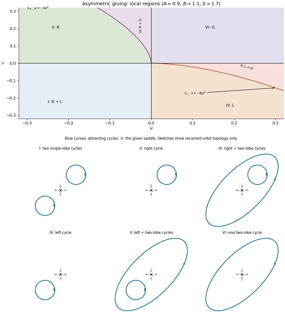
Parameter regions and schematic phase portraits for asymmetric planar gluing
. Details. 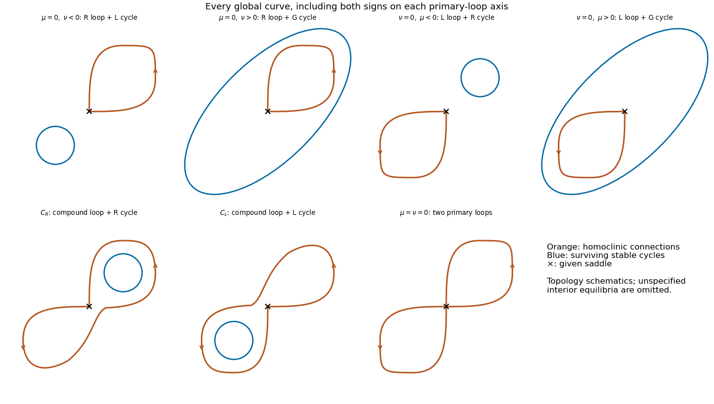


With reflection symmetry, choose and . The two primary homoclinic orbit curves are then encountered simultaneously at . For the return has two attracting single-lobe cycles; for it has one attracting two-lobe cycle. This is the symmetric homoclinic gluing bifurcation: two cycles meet the two saddle loops and are replaced by a cycle traversing both lobes. Since , the saddle equilibrium contracts strongly enough for the nearby cycles to be stable.
One can also use the signed gluing-map reduction . In the symmetric return map it gives . A negative fixed point lifts to two reflection-related flow cycles; a positive fixed point lifts to one period-two orbit of the two-sheet section map, hence one two-lobe flow cycle. This distinction prevents counting the two section intersections as two different flow cycles.
Without reflection symmetry the two splitting parameters are independent. The primary loops occur separately, and the two compound curves bound small coexistence wedges where a single-lobe and a two-lobe cycle are both stable. Thus the six-region picture is the generic two-parameter unfolding of the symmetric gluing event. The simultaneous encounter of both primary loops is codimension two for a general planar flow but codimension one in the reflection-symmetric family. The contraction argument applies to the small return domain; it makes no assertion that a globally arbitrary system has only these cycles everywhere.
For , polar coordinates give and ; the remaining amplitude equation is . Interpret in the original complex coordinate, where the phase is undefined.
If , put . The full equilibrium points are . Their eigenvalues areThus is stable for and has a two-dimensional unstable manifold for . The point has a one-dimensional unstable manifold for and is repelling for . On they merge in a saddle-node bifurcation; the simultaneous zero and imaginary eigenvalues at give a fold-Hopf bifurcation.
A steady positive amplitude represents a full periodic orbit, not a full equilibrium. Solving the amplitude equations givesIt exists in the wedge . The transverse amplitude Jacobian matrix has characteristic polynomial . Its two transverse Floquet exponents have negative real part for and positive real part for ; the phase direction supplies the neutral Floquet multiplier one.
The wedge boundaries are Hopf bifurcations at from and from . The left branch is supercritical, producing a stable periodic orbit as loses stability; the right branch is subcritical in the oscillatory subspace, with an unstable periodic orbit on the side where the transverse complex pair of is stable. The real unstable direction of persists throughout. There are no full equilibrium points when , and then excludes a local periodic orbit. The right panel of the bifurcation diagram in part 1(b) shows the primary curves and the perturbed global curve calculated below.
Within the positive-amplitude wedge the reduced periodic orbit equilibrium has amplitude trace and positive determinant . At the transverse pair is imaginary, so the possible secondary event is a Hopf bifurcation of the amplitude equations, corresponding to an invariant torus in the full system.
It is degenerate. Set and . The first integral of the quadratic fold-Hopf amplitude flow isThe amplitude equations have the Hamiltonian system form , , so . At , has a strict local maximum and negative-definite Hessian. Every nearby regular level is a closed amplitude periodic orbit, rather than one isolated orbit selected by nonlinear damping. Adding the rotating phase gives an entire family of invariant tori; the full motion is quasiperiodic or periodic according to the phase advance during one amplitude period.
For , the amplitude vector field has constant divergence . The Bendixson-Dulac theorem rules out closed amplitude trajectories in the physical simply connected half-plane . Hence there is no ordinary branch of isolated invariant tori on either side in this quadratic system. The secondary event has vanishing radial saturation coefficients; its imaginary linear pair alone does not establish a nondegenerate torus bifurcation.
With the added term, , while and . The prescribed rescaling yieldswhere primes denote . In the limit , the first integral is , since , .
Write . The physical amplitude half-plane is , with of either sign; it is the radial variable , not the axial variable , that is nonnegative. The centre equilibrium is , at . The boundary saddle equilibria are , both at . For , the contours are nested closed curves around the centre. The level consists of the boundary and the interior arcOn the axis , giving a heteroclinic orbit from to . On the arc , giving the reverse heteroclinic orbit. Together they form a heteroclinic cycle. The other parts of the zero level and negative levels give nonclosed trajectories outside this bounded region. The requested contour sketch is shown in the physical radial half-plane.
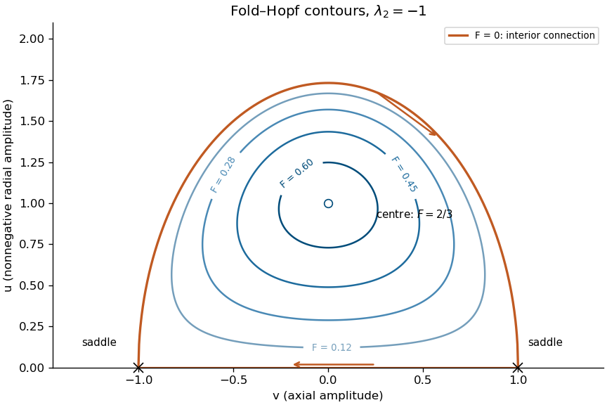
Conserved amplitude contours and the heteroclinic cycle of the quadratic fold–Hopf system
. Details. 
For the perturbed amplitude equations, direct differentiation of the first integral givesThe axis connection contributes zero since . On the unperturbed interior heteroclinic orbit, and , so the first-order change isThe substitution givesConsequentlyThe simple zero of this Melnikov energy-balance method calculation gives the heteroclinic splitting of a fold-Hopf amplitude cycle:This is a leading persistence curve, not an exact parameter equality for the perturbed orbit. It lies between the two primary Hopf bifurcation curves near the origin and on the negative- side of the secondary torus curve . With the added term the primary Hopf bifurcation curves themselves shift to .
The sign of the amplitude balance also identifies the local torus branch. Over a small closed limiting contour, . Its enclosed-area form sets equal to minus the area-average of . This average tends to zero at the centre and to at the heteroclinic cycle. Near the centre, negative attracts trajectories toward the stable amplitude equilibrium; outside a zero-balance contour, decreases and the amplitude excursion grows. Thus the secondary bifurcation creates an unstable invariant torus on the stable-periodic-orbit side. Its continuation reaches the global connection as the balance tends to . The bifurcation diagram distinguishes this perturbed connection from the entire degenerate family present in the unperturbed system.
The normal form is invariant under . This continuous rotational symmetry makes the axis invariant and reduces the nontrivial geometry to two amplitude variables. The axis connection from to persists without parameter tuning, while rotating the outer connection produces a family of connections from back to . A two-dimensional autonomous amplitude flow cannot by itself produce the proposed saddle-focus return chaos: symmetry reduction hides the phase-dependent reinjection needed for that mechanism.
Generic higher-order terms need not retain this exact rotational symmetry. A normal form can preserve it to a finite truncation order while the full equations have small symmetry-breaking remainders. These unfold the special connection geometry into phase-dependent returns; nearby parameter curves can contain homoclinic orbits to a saddle-focus, and the Shilnikov bifurcation mechanism becomes available. Their exact placement depends on the omitted terms and is not fixed by the displayed truncation alone.
For example, at the perturbed positive-axis saddle, the real unstable eigenvalue is and the stable complex pair has real part . Near the calculated connection curve , the contracting ratio isThis is the positive-saddle-value regime, explaining why the relevant saddle-focus return can be expanding.
In the Shilnikov return map, take a positive return coordinate and , with nondegenerate . At the connection parameter , the fixed point condition isThe right side tends to zero, whereas the phase passes through infinitely many oscillations as . Hence there are infinitely many positive fixed points accumulating at zero, with logarithmically spaced amplitudes. For these points,whose magnitude tends to infinity along the accumulating fixed-point sequence. They represent long-period saddle periodic orbits of the full return, with period growing like , rather than infinitely many stable cycles.
Successive turning branches of this oscillatory return can stretch and fold across suitable intervals. The full saddle-focus Poincaré return map then admits invariant Smale horseshoes and chaotic itineraries near a generic homoclinic orbit at a Shilnikov bifurcation. Varying unfolds accumulating saddle-node and period-doubling events. Whether any resulting invariant set attracts trajectories depends on the other return direction and the omitted terms; the leading scalar map alone does not prove a chaotic attractor for every perturbation. Its domain also excludes negative iterates, which leave the chosen return branch. The degeneracies or would remove the oscillatory mechanism, so the conclusion uses generic, genuinely saddle-focus reinjection.
Articles by others on the same topic
There are currently no matching articles.