There are genuine normalization inconsistencies in this PDF. In the standard linearized chord diagram model , time gives edges and total vertex degree , with self-loops counted twice. The paper calls the number of edges. Its right-endpoint hint also uses rather than . These cannot both describe the standard model; part (c)'s exponent is consequently inconsistent as well. We give the definition, prove the alternative construction and its limits, and explicitly identify the corrected conclusion rather than infer an invalid constant from the printed hint.
Start from the empty graph at time zero, or from one vertex with one self-loop at time one. To obtain from , add vertex and an edge directed from to , whereA self-choice creates a self-loop. The old vertex degrees sum to , so these probabilities sum to one. This is exact preferential attachment, including the outward half of the new edge as weight one for the new vertex; it is not a rule normalized by or a process adding two edges at each step. The degree of a vertex here is its total incoming plus outgoing vertex degree. The construction in part (a) has exactly one chord per vertex and makes the edge-count discrepancy explicit.
Draw independent pairs of independent uniform random variables on . In each pair call the minimum and maximum , then relabel whole pairs so . Merge all endpoints in into vertex , with , and join the blocks containing the two endpoints of each pair, orienting from the right endpoint to the left. Self-loops are retained. This gives the uniform linearized chord diagram representation.
Before ordering, a pair has joint density on . Consequently its maximum has distribution and density ; conditional on , its minimum is uniform on . Independence and relabelling give the equivalent precise descriptionEvery one of the relative orderings of the independently drawn labelled endpoints has the same probability. After forgetting pair labels and within-pair labels, each matching of ordered points is produced by orderings. Thus its matching is uniform among the pairings.
To prove equivalence with the recursive graph law, remove the last endpoint and its mate from a uniform pairing. The remaining ordered points have a uniform -pairing, and the mate's old rank is uniform among the possible ranks, independently of that smaller pairing. Conversely insert the mate into a uniformly chosen one of its gaps, and pair it with the new final endpoint. For each old vertex block, the number of gaps assigned to it is exactly the number of endpoints already in that block, hence its old total vertex degree. These are the gaps immediately before each endpoint of that block. The last gap, after the last old endpoint, makes both new endpoints belong to the new final block and produces a self-loop. Therefore the attachment probabilities are for old vertices and for the new one. Induction proves the continuous construction and the recursive LCD model have the same distribution. Inserting a left endpoint into an old block raises exactly that vertex's vertex degree without splitting any old block.
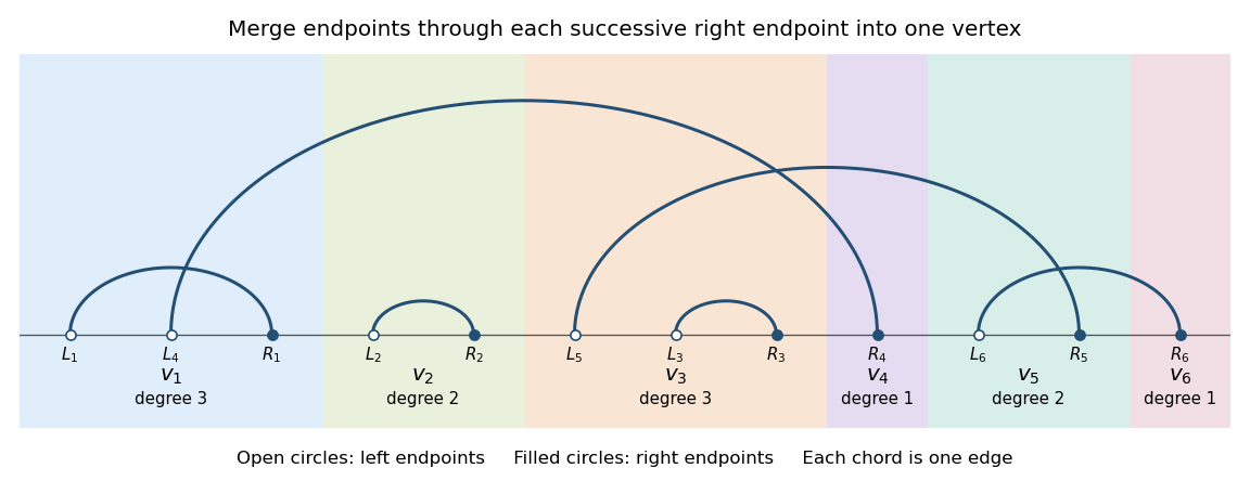
A linearized chord diagram with six vertex blocks, six edges and loops counted twice in the block degrees
. Details. 
The first right endpoint is the smallest of independent pair maxima. A maximum exceeds with probability , so for ,Taking the limit gives the requested, correctly normalized resultThus converges to a continuous nonnegative limit with survival function . In particular the scaled first right endpoint is tight. This calculation uses maxima of pairs, not the first order statistic of all individual endpoints, which would have a different scale. The converted TeX loses the formula in this part; the displayed limit has been recovered directly from the PDF.
First prove the concentration statement with its correct scale. Let , the th uniform order statistic. The number of sample points at most is . Therefore means , and means , up to probability-zero ties. Take and . Applying Chernoff bounds at gives, for an absolute and sufficiently large ,When the upper endpoint exceeds one its upper-tail event is empty. A union bound makes the total failure probability for all at most . On this event,where integral comparison gives .
The first vertex block has right endpoint and always contains , so its initial chord contributes vertex degree two. All its other endpoints are those with that fall below . Conditional on the right endpoints, these events are independent with probabilities . ThusThe fewer than early summands contribute at most to this conditional mean. For the rest, the uniform estimate and uniform tightness of giveTo control the actual fluctuations without assuming unconditional independence, restrict to the concentration event and . Then . Conditional Chebyshev inequality bounds the probability of a deviation exceeding by . The discarded endpoint event has limiting probability ; let . ThereforeSince has a continuous distribution, the corrected first-vertex degree in the LCD model tail isThis disproves the printed exponent for . The hint's factor is independently contradicted at : its proposed upper bound tends to , whereasThus the printed concentration event has probability tending to zero, not one. Replacing its by leads to the proven exponent . The exponent would instead arise for , but then the graph has vertices and the part (b) endpoint limit at becomes . It cannot repair all the printed claims with one convention. The literal part (c) is false for the named model; the full corrected limit and the source of the discrepancy are established above.
Articles by others on the same topic
There are currently no matching articles.