Write , and put , for . Counting the -subsets of the events that occur gives . Set for . The Jordan-Bonferroni exact-occurrence inequalities areHere is an integer. To prove both bounds, evaluate the truncated expression before taking its expectation. At an integer value it equalsFor this is one. For , Pascal's identity, or an induction on , givesFor the original expression is zero. Thus its difference from is everywhere nonnegative for even and nonpositive for odd . Taking expectations proves the inequalities, including .
For a general nonnegative integer-valued random variable, define its factorial moment by , where is the falling factorial and . The same pointwise calculation applies to , so putEvery required moment is finite under the given limit assumption: eventual finiteness of higher factorial moments implies finiteness of the lower ones. The neighbouring upper and lower bounds differ in absolute value byThe last ratio tends to one, and the first factor involving the moment tends to zero. Since lies between every two such neighbouring bounds, each tends to it. Consequently the factorial-moment inversion isThis proves convergence of the signed series without an unjustified interchange with an expectation.
For any prescribed , take for , with . Since and , the two moment sums have tails comparable respectively to and . Thus but , as required.
Take and , as required for the displayed sparse scaling and the later normalization. A strictly balanced graph satisfies for every proper nonempty subgraph . This forces to be connected and to have no isolated vertices: otherwise a component of at least the average density, or deletion of the isolated vertices, violates strict balance. Copies here are subgraphs, not induced subgraphs.
For fixed , the factorial moment counts ordered -tuples of distinct copies all present in the binomial random graph. The contribution of vertex-disjoint copies is exactlyThe factor removes the multiple embeddings of each copy coming from its graph automorphisms. For an overlapping tuple, let be its union. There are placements of each fixed union type, and the probability its edges are present is . When adding a copy meeting the earlier union in vertices and edges, the exponent changes byIt is strictly negative if this intersection is a proper nonempty subgraph, and zero only for an empty intersection or a whole copy. In particular the first vertex-overlapping copy has a proper nonempty intersection: the preceding copies are vertex-disjoint, and a connected copy contained in their union would have to equal one of them, contrary to distinctness. Its contribution is therefore strictly negative; later additions cannot undo that loss. Only finitely many union types occur for fixed , so their total contribution is . We have proved all the factorial moment limits, and the allowed factorial-moment criterion for Poisson convergence givesThis is the Poisson limit for strictly balanced subgraph counts.
The pendant-edge graph has density , whereas its proper core has density . Thus is not strictly balanced. The complete graph is strictly balanced, with 24 graph automorphisms, so at its copy count tends to .
Every copy has a unique four-vertex clique core and one selected edge joining it to a fifth vertex. For any four-set , let count the ambient edges between and its complement. Then , with mean . It is independent of the internal edges determining whether is a clique. Choose . A Chernoff bound and a union bound giveTherefore, simultaneously for every actual core, its number of pendant extensions is . Extra ambient edges cause no overcount: each selected seven-edge subgraph has exactly one core and one pendant edge. Summing over the cores yieldsbecause is uniformly tight. This is the pendant extensions of sparse clique copies mechanism. For , neither endpoint of is an integer, and its only nonnegative integer is . Convergence in distribution consequently givesThe positive- assumption matters: the quotient printed in the question is undefined when .
If the random k-out graph with is disconnected, one of its connected components of a graph has size . The lower bound follows because every vertex chooses two distinct neighbours inside its component. For a specified -set , absence of crossing edges requires every choice at a vertex in to stay in , and every choice outside to stay outside. Independence of choices at different vertices gives exactlyFor , the two ratios are at most and . Indeed each of the factors , , is at most , and the complementary statement is identical. Put . The binomial coefficient bound follows by bounding the probability of successes in by one. Thus the union bound givesFor , the last summands are at most , whose sum from three tends to zero. For , they are at most , again summing to zero. ThereforeThe proof bounds all possible small components rather than assuming the dependent undirected edges behave like a binomial random graph.
At each vertex independently, take a uniformly random permutation of the other vertices. Use its first two entries for the two-out choices and its first entries for the -out choices. Every unordered choice set has the prescribed uniform distribution, and choices at different vertices remain independent. This couples the random k-out graphs so that on the same vertex set. Adding edges cannot destroy graph connectivity. ConsequentlyThis establishes connectivity of random k-out graphs for every fixed allowed .
Relative to a filtration , a martingale is an adapted process of integrable random variables satisfying . With no separate filtration specified, take the natural filtration . For deterministic increment bounds , the Hoeffding-Azuma inequality statesTo prove it, let . For , convexity on givesIts conditional expectation is at most . The last inequality follows by integrating for and using evenness. If the bound is immediate. Conditional iteration now yields . The exponential Markov inequality, minimized at , bounds the upper tail by the displayed exponential without the factor two. Apply it to and use the union bound for the two-sided assertion. When every , the deviation probability is zero.
For the chromatic number of a binomial random graph, put , , and . We prove matching bounds; treating suffices. A colour class is an independent set, so . For with fixed , the expected value of the number of independent -sets isThe first moment method gives with probability tending to one. Choosing sufficiently small then gives for all sufficiently large on that event.
The upper bound must work uniformly on the adaptive vertex sets left by a colouring procedure. SetFor a specified -set , its complement graph has distribution . Let count its -cliques, count distinct ordered pairs sharing an edge, and be the maximum edge-disjoint clique packing. The allowed clique-count estimates at this value of giveThe overlap quantity, if the diagonal is included, has the exact expression after division by ; the same bound holds. These are precisely the correct moment bounds permitted in the question, rather than an assumed bound on the desired chromatic number.
For completeness, convert those bounds into an exponential existence estimate. In the clique conflict graph the vertices are the existing cliques, with an edge between each conflicting pair. A random ordering keeps every vertex that precedes all its neighbours. No two retained vertices are adjacent. Their mean number is by the Cauchy-Schwarz inequality. Thus, with a zero ratio when ,The middle inequality follows from . Toggling one ambient edge changes by at most one: at most one member of a packing uses it. Reveal the independent edges successively and form the edge-exposure martingale for . Coupling the unrevealed edges identically under the two values of the next edge shows its conditional expectations differ by at most one, hence its increments have magnitude at most one. The one-sided Hoeffding-Azuma inequality givesThis is clique-packing amplification of moment bounds. A union bound over all -sets is now strong enough:since . Thus every such set contains an independent set of size . Repeatedly remove and colour one whenever at least vertices remain; then colour each of the fewer than remaining vertices separately. This greedy colouring by removing independent sets uses at mostChoose so . Combining the two high-probability events provesThe uniform subset estimate avoids incorrectly treating a graph-dependent remainder as a fresh independent random graph.
Let denote the generation- type-count vector, and let from a single type- ancestor. Every type- child independently has probability of having descendants in generation . For a Poisson random variable with mean , . Independence across child types therefore givesThe events of nonempty successive generations decrease. Each individual has finitely many children almost surely, so the total tree is infinite precisely when no generation is empty. Consequently , the actual survival probability of a branching process. Continuity of yieldsThe map is coordinatewise increasing on nonnegative vectors. Every nonnegative fixed point automatically lies in , since its coordinates equal with finite . Hence and, by induction, . Taking limits proves in every coordinate, so is the greatest nonnegative solution, not merely some fixed point. This argument applies without irreducibility assumptions to the multitype Poisson branching process.
Use row vectors for population counts. Given , independent reproduction has conditional mean . Starting from , induction gives . Summing all child types, the expected size of generation isThis also covers , using . All these finite-generation expectations are finite because the matrix is finite with finite entries.
The necessary and sufficient condition iswhere is the spectral radius of the nonnegative matrix. No irreducibility is required. We use the given nonnegative-vector characterization of its Perron eigenvalue.
For necessity, suppose is the survival fixed point and let . Since for every , its equation gives for every . There are finitely many such coordinates, soOutside the inequality still holds, because its right side is zero and its left side is nonnegative. The provided Perron–Frobenius theorem characterization therefore gives . In particular survival is impossible at for this Poisson offspring law.
Conversely suppose . The given characterization supplies a nonzero with ; normalize it so . For sufficiently small ,For example any works. Coordinates with satisfy the inequality automatically. Starting at , iterate . Monotonicity makes the sequence increase, and takes nonnegative vectors into , so it converges to a fixed point . Part (a) gives , proving survival from at least one type. This proves the spectral survival criterion for multitype Poisson branching for reducible as well as irreducible reproduction matrices.
There are genuine normalization inconsistencies in this PDF. In the standard linearized chord diagram model , time gives edges and total vertex degree , with self-loops counted twice. The paper calls the number of edges. Its right-endpoint hint also uses rather than . These cannot both describe the standard model; part (c)'s exponent is consequently inconsistent as well. We give the definition, prove the alternative construction and its limits, and explicitly identify the corrected conclusion rather than infer an invalid constant from the printed hint.
Start from the empty graph at time zero, or from one vertex with one self-loop at time one. To obtain from , add vertex and an edge directed from to , whereA self-choice creates a self-loop. The old vertex degrees sum to , so these probabilities sum to one. This is exact preferential attachment, including the outward half of the new edge as weight one for the new vertex; it is not a rule normalized by or a process adding two edges at each step. The degree of a vertex here is its total incoming plus outgoing vertex degree. The construction in part (a) has exactly one chord per vertex and makes the edge-count discrepancy explicit.
Draw independent pairs of independent uniform random variables on . In each pair call the minimum and maximum , then relabel whole pairs so . Merge all endpoints in into vertex , with , and join the blocks containing the two endpoints of each pair, orienting from the right endpoint to the left. Self-loops are retained. This gives the uniform linearized chord diagram representation.
Before ordering, a pair has joint density on . Consequently its maximum has distribution and density ; conditional on , its minimum is uniform on . Independence and relabelling give the equivalent precise descriptionEvery one of the relative orderings of the independently drawn labelled endpoints has the same probability. After forgetting pair labels and within-pair labels, each matching of ordered points is produced by orderings. Thus its matching is uniform among the pairings.
To prove equivalence with the recursive graph law, remove the last endpoint and its mate from a uniform pairing. The remaining ordered points have a uniform -pairing, and the mate's old rank is uniform among the possible ranks, independently of that smaller pairing. Conversely insert the mate into a uniformly chosen one of its gaps, and pair it with the new final endpoint. For each old vertex block, the number of gaps assigned to it is exactly the number of endpoints already in that block, hence its old total vertex degree. These are the gaps immediately before each endpoint of that block. The last gap, after the last old endpoint, makes both new endpoints belong to the new final block and produces a self-loop. Therefore the attachment probabilities are for old vertices and for the new one. Induction proves the continuous construction and the recursive LCD model have the same distribution. Inserting a left endpoint into an old block raises exactly that vertex's vertex degree without splitting any old block.
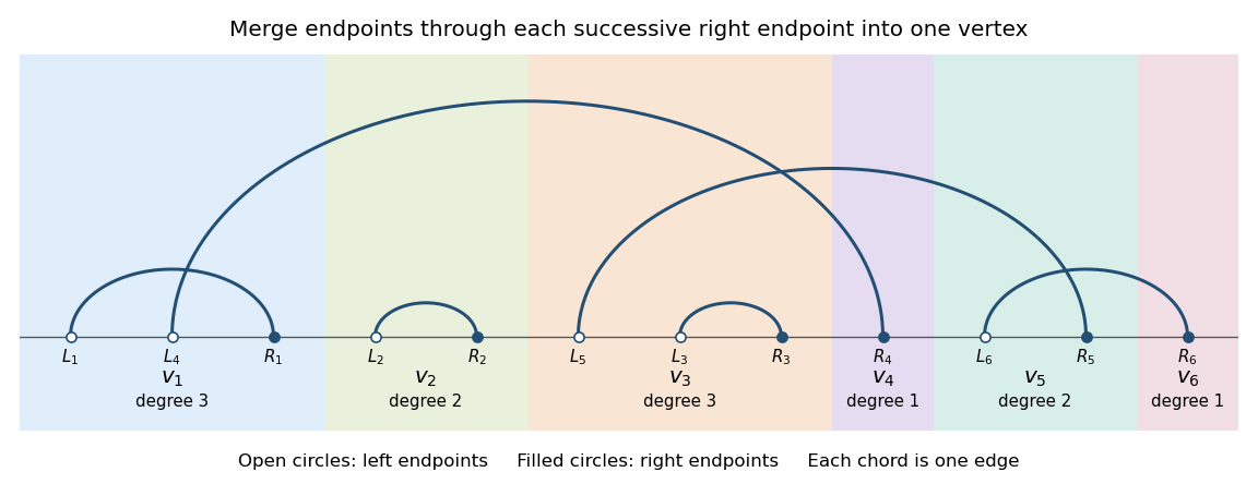
A linearized chord diagram with six vertex blocks, six edges and loops counted twice in the block degrees
. Details. 
The first right endpoint is the smallest of independent pair maxima. A maximum exceeds with probability , so for ,Taking the limit gives the requested, correctly normalized resultThus converges to a continuous nonnegative limit with survival function . In particular the scaled first right endpoint is tight. This calculation uses maxima of pairs, not the first order statistic of all individual endpoints, which would have a different scale. The converted TeX loses the formula in this part; the displayed limit has been recovered directly from the PDF.
First prove the concentration statement with its correct scale. Let , the th uniform order statistic. The number of sample points at most is . Therefore means , and means , up to probability-zero ties. Take and . Applying Chernoff bounds at gives, for an absolute and sufficiently large ,When the upper endpoint exceeds one its upper-tail event is empty. A union bound makes the total failure probability for all at most . On this event,where integral comparison gives .
The first vertex block has right endpoint and always contains , so its initial chord contributes vertex degree two. All its other endpoints are those with that fall below . Conditional on the right endpoints, these events are independent with probabilities . ThusThe fewer than early summands contribute at most to this conditional mean. For the rest, the uniform estimate and uniform tightness of giveTo control the actual fluctuations without assuming unconditional independence, restrict to the concentration event and . Then . Conditional Chebyshev inequality bounds the probability of a deviation exceeding by . The discarded endpoint event has limiting probability ; let . ThereforeSince has a continuous distribution, the corrected first-vertex degree in the LCD model tail isThis disproves the printed exponent for . The hint's factor is independently contradicted at : its proposed upper bound tends to , whereasThus the printed concentration event has probability tending to zero, not one. Replacing its by leads to the proven exponent . The exponent would instead arise for , but then the graph has vertices and the part (b) endpoint limit at becomes . It cannot repair all the printed claims with one convention. The literal part (c) is false for the named model; the full corrected limit and the source of the discrepancy are established above.
Articles by others on the same topic
There are currently no matching articles.