Use the Wirtinger derivatives and . In particular . Let , and , so the printed differential form is . Since and ,Thus the exterior derivative isBecause never vanishes and , this proves both directions: is a closed differential form if and only if . The latter is the modified Helmholtz equation for positive . The associated global relations on a bounded region are, for every nonzero spectral parameter,The boundary orientation is positive, by Stokes theorem. Each admissible spectral parameter gives a separate identity between the traces. Interchanging and gives the dual family, equivalently the same family at with an overall minus sign. No assumption that is real is needed.
For later use with , as in the remaining parts, make the global relation explicit in the first quadrant. PutLet , and , . These normals are inward-coordinate derivatives. The bottom is traversed from zero to infinity and the left side from infinity to zero. Their oriented spectral integrals areHere is analytic for and for , with suitable boundary limits. Indeed and for . On their common third quadrant, both exponential weights decay. Apply the finite-domain relation to expanding rectangles; sufficient decay of the solution and traces eliminates the distant edges. This derivesThe limiting relations on the negative real and negative imaginary axes will remove the unknown derivative traces.
The modified Helmholtz closed spectral one-form is exact in the simply connected quadrant. Writing its primitive as gives the compatible first-order equationsTheir compatibility is precisely the PDE already proved in part (a). Set . Construct three primitives: starts at the corner, starts at the infinite end of a horizontal line through the point, and starts at the infinite end of a vertical line. More explicitly,Path independence follows from closedness. The two infinite primitives exist in the lower and left spectral half-planes respectively. In their common third quadrant they coincide, because the global relation makes the difference of the two basepoint integrals zero.
Choose a sectionally analytic spectral function by using in quadrant I, in quadrant II and in quadrants III and IV. It has no jump across the negative axes. Let and , both oriented outward. With plus denoting the left side of an oriented ray, the two remaining jumps areFor example, on the jump is , the primitive around the bottom boundary; on it is , the left boundary traversed downward. This fixes both orientations and signs of the Riemann-Hilbert problem.
Integration by parts in the infinite primitive formulas, or in the finite primitive with its decaying basepoint contribution, givesFor instance the horizontal formula has leading value , which tends to at infinity and at zero; the vertical formula has leading value with the same limits. These expansions hold in closed subsectors, with the boundary limits obtained by oscillatory regularization. Along , damps with at both spectral ends; along , it damps with . Thus the ray integrals converge in the interior and small and large spectral circles can be removed.
Solve the additive Riemann-Hilbert problem by a Cauchy integral formula, normalized at infinity:The Sokhotski–Plemelj theorem gives the stated jumps. The difference between this expression and the constructed primitive is analytic across both rays, bounded at zero and vanishes at infinity; the Liouville theorem makes that difference zero. Evaluate at zero, where . The difference between the two spectral normalizations is , hence the quadrant modified Helmholtz spectral reconstruction isThe factor is essential. A useful independent normalization check is to write on the real ray, so and . On the imaginary ray write , and . The formula becomesEach hat here is a half-line Fourier transform. This is exactly the spectral form of Green second identity with the decaying full-plane fundamental solution. The representation still contains both value and derivative traces; the next part eliminates the latter.
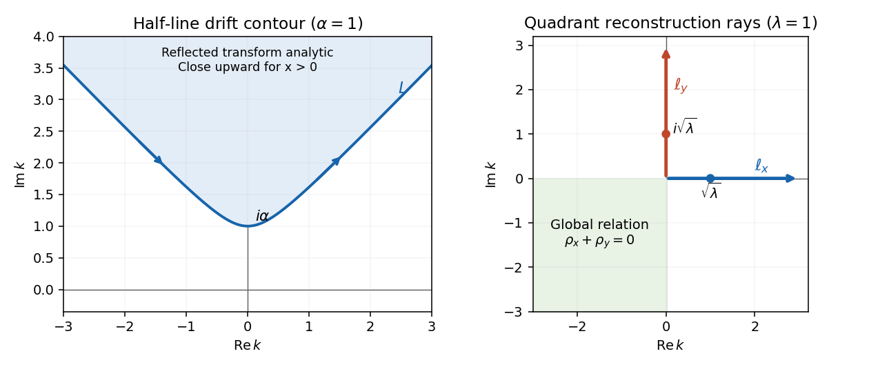
Oriented half-line drift contour and quadrant modified Helmholtz reconstruction rays with their analytic and global-relation domains
. Details. 
Now and . Define their Fourier sine transformsFirst make the elimination from the global relations explicit. Write and . For , set . Apply the relation of part (a) at the two negative real spectral points and . They have the same and opposite . Subtracting cancels the left derivative transform, and givesLikewise use , which have the same and opposite . Their difference givesThus both unknown normal traces have sine transforms determined by the given data. The reciprocal symmetries of the dispersion curve, rather than an arbitrary assumption about an unknown trace, perform the elimination.
Here is a direct way to finish that elimination in the integral representation of part (b). Its full-plane kernel has Fourier representationand solves . Form the four-image kernelFor , the three reflected source points are outside the quadrant. Their boundary integrals against the solution vanish by Green second identity; spectrally these are superpositions of the same reflected global relations used above. Thus replacing by in part (b) does not change . But vanishes on either boundary, so all terms multiplying unknown normal traces disappear. The remaining inward kernel derivatives reconstruct the value:Differentiate the displayed spectral kernel and combine positive and negative . The bottom derivative is , and the left derivative is the corresponding expression with interchanged. This derives the quadrant modified Helmholtz Dirichlet Poisson formula, entirely in known data:It is an integral on the same complex dispersion curve. To display the requested complex -plane contours explicitly, let and as before. On the real ray above , , and . On the imaginary ray above , , and . ConsequentlyBoth contours are oriented outward, and the sine-transform arguments on them are positive real numbers. No unknown boundary transform remains.
Every integrand solves , because . As with , the first term tends to by Fourier sine inversion and the second tends to zero by exponential convergence; the left trace follows symmetrically. Although the two separate contributions may have different corner limits, their sum is continuous at the corner when . For example, the local constant-data corner contributions are the complementary angular harmonic weights, whose sum is one; the mass term is lower order under corner rescaling. Equivalently, subtract a smooth local lifting with the common corner value and use the zero-trace quadrant Green function to obtain a continuous remainder. Decay and uniqueness follow from the positive mass and the weak maximum principle, or from the positive energy identity for a difference with zero boundary data.
Articles by others on the same topic
There are currently no matching articles.