Extend by zero to . Its ordinary Fourier transform is precisely the half-line transform , so Fourier inversion gives the real-axis term for every interior point . At the zero extension can have a jump; the interior inversion is the assertion needed here.
Write . The contour is the upper branch of a hyperbola,with increasing from to . In the region above it, has nonpositive imaginary part. Therefore is analytic there: its defining integral has factor and converges for a sufficiently decaying . Smoothness and integration by parts also give away from bounded spectral sets.
For an interior spatial point , the factor decays exponentially as . Truncate the hyperbolic contour and close it above, using the Cauchy integral theorem; the closing segments vanish by this decay and the transform estimate. No poles occur in the enclosed region. Consequently the half-line drift null contour identity isAdding any constant multiple of zero to Fourier inversion proves the proposed inversion, for every . Oscillatory real-axis inversion may be understood by a Gaussian cutoff followed by its usual limit. The same contour argument allows a spectral multiplier analytic above with polynomial growth, because the exponential still controls the closing paths. We will need this slight extension for derivative boundary data.
Set and , so . For boundary traces , defineThe Half-range Fourier transform of the equation is obtained by two integrations by parts:Solving this scalar equation gives the drift-diffusion half-line global relationIn particular the reflected relation is valid on , since there.
In the region between the real axis and , . Thus a boundary contribution admits an upward contour deformation from the real axis to . Large-contour estimates follow from the spatial exponential and the time integral; at the upper time endpoint one can integrate in time once or use a small contour displacement. The initial-data transform is retained on the real axis. Hence, if , ordinary inversion first givesFor the Dirichlet boundary condition, take . Subtract the null integral of the reflected time-dependent transform, using the inversion from part (a) with . The unknown derivative transform cancels because . This derives the Dirichlet spectral formula for half-line constant drift:Only initial and prescribed boundary data occur in this expression.
For the Neumann boundary condition, take . The reflected global relation reads . Solve for and substitute it in the preliminary representation. The leftover term is a null integral with multiplier , analytic above ; its pole at zero is below the contour. Thus the Neumann spectral formula for half-line constant drift isThere is no residue from the origin, since this elimination never moves the contour across it. The given derivative is the inward-coordinate derivative , not the outward derivative . The initial compatibility for this case is .
The Dirichlet spectral formula for half-line constant drift can be checked both spectrally and through its heat kernel. For , each factor solves the differential equation, since . Differentiating the upper limit in introduces onlyThis vanishes by closing upward for , or by recognizing the polynomial Fourier multiplier as a distribution supported at . Thus differentiation under regularized contours, followed by the smooth interior limit, proves the PDE. At the boundary transform vanishes and the reflected initial-data integral is zero by part (a), leaving Fourier inversion of .
For a direct verification of the boundary limit, evaluate the contour integrals. LetThe real-axis Gaussian Fourier transform gives this kernel. In the reflected initial term, , so a valid contour deformation gives . The boundary integral gives . Consequently the same solution iswhereInterchange of the space or time integrals with the spectral integral can first be performed with cutoffs; the displayed Gaussian kernels justify their removal for the stated smooth decaying data. The possible exponential is compensated by Gaussian decay, so exponential decay of is not an extra assumption.
At , , so the initial-data contribution has zero boundary trace. The kernel is a time approximate identity as . Indeed it is the standard positive heat boundary kernel multiplied by . The standard kernel has total mass one on , as the substitution shows; its mass on is . The additional factor tends to one uniformly on sufficiently short time intervals as , so for fixed . Continuity of and the vanishing tail then giveFor fixed , the first kernel tends to a point mass at , the reflected kernel is exponentially small as , and the boundary-forcing integral is also exponentially small. This independently proves . The compatibility supplies continuity at the initial corner.
Use the Wirtinger derivatives and . In particular . Let , and , so the printed differential form is . Since and ,Thus the exterior derivative isBecause never vanishes and , this proves both directions: is a closed differential form if and only if . The latter is the modified Helmholtz equation for positive . The associated global relations on a bounded region are, for every nonzero spectral parameter,The boundary orientation is positive, by Stokes theorem. Each admissible spectral parameter gives a separate identity between the traces. Interchanging and gives the dual family, equivalently the same family at with an overall minus sign. No assumption that is real is needed.
For later use with , as in the remaining parts, make the global relation explicit in the first quadrant. PutLet , and , . These normals are inward-coordinate derivatives. The bottom is traversed from zero to infinity and the left side from infinity to zero. Their oriented spectral integrals areHere is analytic for and for , with suitable boundary limits. Indeed and for . On their common third quadrant, both exponential weights decay. Apply the finite-domain relation to expanding rectangles; sufficient decay of the solution and traces eliminates the distant edges. This derivesThe limiting relations on the negative real and negative imaginary axes will remove the unknown derivative traces.
The modified Helmholtz closed spectral one-form is exact in the simply connected quadrant. Writing its primitive as gives the compatible first-order equationsTheir compatibility is precisely the PDE already proved in part (a). Set . Construct three primitives: starts at the corner, starts at the infinite end of a horizontal line through the point, and starts at the infinite end of a vertical line. More explicitly,Path independence follows from closedness. The two infinite primitives exist in the lower and left spectral half-planes respectively. In their common third quadrant they coincide, because the global relation makes the difference of the two basepoint integrals zero.
Choose a sectionally analytic spectral function by using in quadrant I, in quadrant II and in quadrants III and IV. It has no jump across the negative axes. Let and , both oriented outward. With plus denoting the left side of an oriented ray, the two remaining jumps areFor example, on the jump is , the primitive around the bottom boundary; on it is , the left boundary traversed downward. This fixes both orientations and signs of the Riemann-Hilbert problem.
Integration by parts in the infinite primitive formulas, or in the finite primitive with its decaying basepoint contribution, givesFor instance the horizontal formula has leading value , which tends to at infinity and at zero; the vertical formula has leading value with the same limits. These expansions hold in closed subsectors, with the boundary limits obtained by oscillatory regularization. Along , damps with at both spectral ends; along , it damps with . Thus the ray integrals converge in the interior and small and large spectral circles can be removed.
Solve the additive Riemann-Hilbert problem by a Cauchy integral formula, normalized at infinity:The Sokhotski–Plemelj theorem gives the stated jumps. The difference between this expression and the constructed primitive is analytic across both rays, bounded at zero and vanishes at infinity; the Liouville theorem makes that difference zero. Evaluate at zero, where . The difference between the two spectral normalizations is , hence the quadrant modified Helmholtz spectral reconstruction isThe factor is essential. A useful independent normalization check is to write on the real ray, so and . On the imaginary ray write , and . The formula becomesEach hat here is a half-line Fourier transform. This is exactly the spectral form of Green second identity with the decaying full-plane fundamental solution. The representation still contains both value and derivative traces; the next part eliminates the latter.
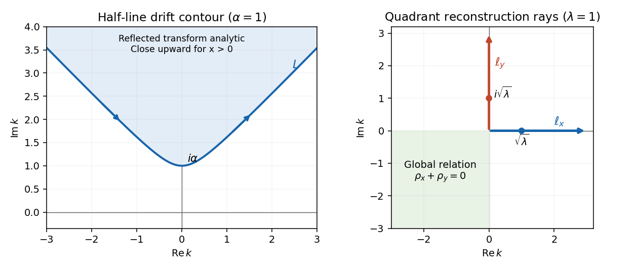
Oriented half-line drift contour and quadrant modified Helmholtz reconstruction rays with their analytic and global-relation domains
. Details. 
Now and . Define their Fourier sine transformsFirst make the elimination from the global relations explicit. Write and . For , set . Apply the relation of part (a) at the two negative real spectral points and . They have the same and opposite . Subtracting cancels the left derivative transform, and givesLikewise use , which have the same and opposite . Their difference givesThus both unknown normal traces have sine transforms determined by the given data. The reciprocal symmetries of the dispersion curve, rather than an arbitrary assumption about an unknown trace, perform the elimination.
Here is a direct way to finish that elimination in the integral representation of part (b). Its full-plane kernel has Fourier representationand solves . Form the four-image kernelFor , the three reflected source points are outside the quadrant. Their boundary integrals against the solution vanish by Green second identity; spectrally these are superpositions of the same reflected global relations used above. Thus replacing by in part (b) does not change . But vanishes on either boundary, so all terms multiplying unknown normal traces disappear. The remaining inward kernel derivatives reconstruct the value:Differentiate the displayed spectral kernel and combine positive and negative . The bottom derivative is , and the left derivative is the corresponding expression with interchanged. This derives the quadrant modified Helmholtz Dirichlet Poisson formula, entirely in known data:It is an integral on the same complex dispersion curve. To display the requested complex -plane contours explicitly, let and as before. On the real ray above , , and . On the imaginary ray above , , and . ConsequentlyBoth contours are oriented outward, and the sine-transform arguments on them are positive real numbers. No unknown boundary transform remains.
Every integrand solves , because . As with , the first term tends to by Fourier sine inversion and the second tends to zero by exponential convergence; the left trace follows symmetrically. Although the two separate contributions may have different corner limits, their sum is continuous at the corner when . For example, the local constant-data corner contributions are the complementary angular harmonic weights, whose sum is one; the mass term is lower order under corner rescaling. Equivalently, subtract a smooth local lifting with the common corner value and use the zero-trace quadrant Green function to obtain a continuous remainder. Decay and uniqueness follow from the positive mass and the weak maximum principle, or from the positive energy identity for a difference with zero boundary data.
Write , with , and rotate the plane into the line coordinatesThus and , agreeing with the directed-line geometry in the PDF. Direct substitution, rather than a formal complex rotation, gives the directional differential operatorwhere and . If , choose the invertible real-linear complex coordinateThe Wirtinger derivative in this coordinate is , so . Substitution gives the required transformed equation with the same multiplication and source terms. This is a new spectral-dependent spatial coordinate, not the physical used in Question 2.
The complex change of variables is valid for . At , and the operator becomes the real line derivative ; there can be no invertible elliptic complex-coordinate change there. The two limits to this characteristic circle are precisely the boundary values needed in part (b). The expression at is undefined in the printed equation and is treated through its spectral limit, not by substitution.
Keep the coordinates and operator from part (a). The attenuation is known, and the source is to be reconstructed. Put and . The directed forward attenuated Radon transform, for a detector at the positive end of the line, isThis weight accounts for absorption from each emission point to the detector. It is also derived by solving the real transport equation with zero incoming intensity: its outgoing limit is . In particular reversing the line direction generally changes the measurement. The pair reconstructs from full directed data and known ; it does not infer both unknown functions from the same data.
We must specify the sign convention for the projectors. Use the Hilbert transform and the signed Cauchy boundary operatorsThen , and the positive idempotent projectors are and . This is the signed boundary-value convention in the given limits of . To express everything with ordinary complementary projectors, one may instead write , . The given limits becomeBoth depend on the transverse coordinate and direction but are constant along .
The equation supplies an integrating factor:where is the inverse of unattenuated complex transport, normalized to vanish at spatial infinity. To see the normalization and analyticity rather than assume them, let . The complexified transport Cauchy kernel isIn the rotated coordinates, . The identity and the Jacobian prove with exactly this normalization. The denominator cannot vanish for nonzero real off the unit circle. The kernel is analytic separately inside and outside that circle, is at zero and at infinity. Thus and the displayed have the corresponding spectral behavior for the smooth decaying data. In particular at infinity and is bounded, indeed , at zero.
The limiting unattenuated inverse on any smooth decaying input isOne may verify this directly in the rotated Fourier variables: has multiplier , so its inverse has a pole at . As , the positive transverse frequencies have the negative tail primitive and the negative transverse frequencies have the positive past primitive; for these allocations reverse. Splitting with the Fourier projectors yields exactly the two formulas above. Applying them to reproduces the assumed limits of and checks the signs.
Now apply the same limiting inverse to . Because are independent of , its line integral is , while its tail is . HenceThe unknown incomplete line integral cancels in their difference. All remaining quantities are obtained from the measurements and known attenuation:Each projection acts in at fixed , before evaluating and . Pulling a transverse-dependent exponential outside a projector would be incorrect.
The sectionally analytic therefore solves an additive Riemann-Hilbert problem on the counterclockwise unit circle, with the plus value inside. The normalized Cauchy integral formula isThe Sokhotski–Plemelj theorem gives its jump; boundedness at zero and decay at infinity make it unique by the Liouville theorem. Its expansion at infinity isSubstitute into the original equation. The part contributes at order one, the reciprocal derivative and vanish at that order. This derives the projection formula for inverse attenuated Radon transform:Together with the boxed forward transform this is the requested pair. The derivation uses no small-attenuation approximation. For smooth compactly supported data the operations above are justified directly; sufficient integrable decay permits the same limiting construction.
As a normalization check, set . Then , and . Since the line transform is independent of and , the formula reduces tothe full-angle inverse Radon transform. For the radial Gaussian , and , so the reconstructed value at the origin is , checking the factor.
In single-photon emission computed tomography, represents the internal emission density, the known absorption coefficient and the directed detector counts. Each path integral weights a source point by its survival probability to the detector. Thus the attenuated Radon transform is the forward measurement model and its derived inverse reconstructs the emission distribution, providing the mathematical basis of SPECT.
Articles by others on the same topic
There are currently no matching articles.