Past exam of the mathematics course of the University of Cambridge / 2018 / iii / Paper 219 / 4

Write $v={\sigma }_{\mathrm{int}}^2$, $r_s={\sigma }_{O,s}^2$ and $o_s={\hat{O}}_s$. A flat density in $\log \tau$ means $p(\tau )\propto 1/\tau$ with respect to $d\tau$; likewise $p(v)\propto 1/v$. The Jacobian determinant must therefore appear when using the original scale variables. The joint hierarchical Bayesian model kernel, with respect to $d{\mu }_{C}dvd\tau {\prod }_{s}d{o}_{s}d{C}_{s}d{E}_s$, isThis is a kernel, not a normalized joint probability distribution, because the stated priors are improper. Conditioning on $o$ would still require posterior propriety. In fact that check fails here, as shown in part (iii)(c); proper formal full conditionals alone do not repair it. The Gaussian–exponential hierarchical colour model distinguishes the intrinsic normal colour, positive interstellar dust reddening, and measurement noise.

The probabilistic graphical model is the following Directed acyclic graph. The shared hyperparameters lie outside the plate; the plate repeats the local variables for $s=1,\dots ,N$. The observed colour is shaded, and the known error variance $r_s$ is a square.

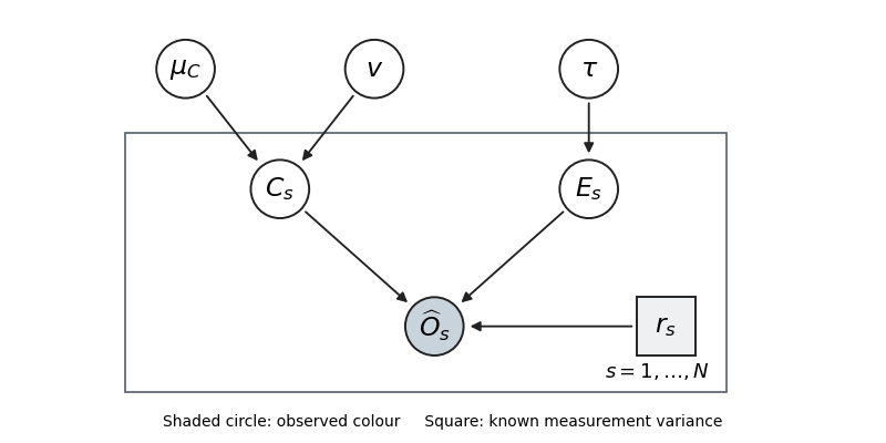
Thus the parent sets are $\boxed{\mathrm{pa}(C_s)=\{{\mu }_C,v\},\mathrm{pa}(E_s)=\{\tau \},\mathrm{pa}(o_s)=\{C_s,E_s,r_s\}}$. Independent hyperparameter prior factors are represented by the three root nodes. With the printed improper priors this is a factorization diagram; it becomes a normalized generative model after proper priors are supplied.

Use the abbreviations in (i). Keeping only terms involving $C_s$ in the joint kernel and completing the square givesConsequently the Gaussian latent-colour update isThese $N$ updates are conditionally independent given the remaining variables. The flat mean prior gives one more normal full conditional:The factorization uses ${\sum }_s(C_s-{\mu }_C{)}^2={\sum }_s(C_s-\overline{C}{)}^2+N({\mu }_C-\overline{C}{)}^2$. Together these are the $N+1$ normal draws in the formal Gibbs sampler.

The terms involving $E_s$ giveCompleting the square produces the truncated normal distributionFor $m=o_s-C_s-r_s/\tau$, its normalized density is $\varphi ((E_s-m)/\sqrt{r_s})/[\sqrt{r_s}\Phi (m/\sqrt{r_s})]$ on $E_s\ge 0$. The exponential prior shifts the untruncated conditional mean downwards before truncation; changing the variance here to the intrinsic variance would be incorrect. These are the other $N$ latent-variable updates of the formal Gibbs sampler.

Keeping the powers and exponentials of $v$ and $\tau$ in the joint kernel gives the two inverse-gamma distributions, using the printed shape–scale convention:Indeed their kernels are $v^{-(N/2+1)}\exp [-{\sum }_s(C_s-{\mu }_C{)}^2/(2v)]$ and ${\tau }^{-(N+1)}\exp [-{\sum }_s{E}_s/\tau ]$. With positive measurement variances and generic continuously drawn latent values, the two scale parameters are positive almost surely. Together with (a),(b), these are all $2N+3$ formal full conditional updates.

There is, however, no joint posterior probability distribution to sample under the stated priors. Integrate out the intrinsic $C_s$ first. For fixed ${\mu }_C,v>0$, the observational marginal density iswhere ${\varphi }_V$ is the centred normal density of variance $V$. Substitute $E=\tau u$. Dominated convergence givesThe convergence is uniform on any compact ${\mu }_C$ interval and any compact positive $v$ interval, since the normal densities are uniformly bounded and continuous there. Hence some such region has $L\ge c>0$ for all sufficiently small $\tau$, andIntegrating over those positive-measure intervals proves that the full normalizing constant is infinite. If all $r_s>0$, the $v\downarrow 0$ boundary also gives a positive marginal likelihood and a divergent $dv/v$ integral at fixed $\tau >0$. Thus $\boxed{\text{the stated joint posterior is improper}}$, even though its generic full conditionals are proper. Apparent stability of a simulated chain cannot establish a nonexistent stationary probability law.

A valid repair that preserves direct sampling is to replace the two log-flat priors by independent proper $v\sim \mathrm{IG}(a_v,b_v)$ and $\tau \sim \mathrm{IG}(a_{\tau },b_{\tau })$, with all four constants positive. The normal and truncated-normal updates remain as above, whileWith positive $r_s$, the flat ${\mu }_C$ prior is then harmless: after integrating it out, the Gaussian measurement likelihood is bounded uniformly over the latent shifts and the scales, and the remaining proper priors integrate to one. A proper prior on ${\mu }_C$ is also possible.

For this repaired model, initialize $v,\tau >0$, $E_s\ge 0$ and finite $C_s,{\mu }_C$. Repeatedly choose one of the $2N+3$ coordinates with fixed positive probabilities and redraw from its full conditional using the latest values. This Random-scan Gibbs sampler preserves the proper target and satisfies detailed balance: for each coordinate, both forward and reverse flows equal the marginal density of the remaining coordinates times the product of the two conditional densities. A systematic full sweep is another invariant scheme, though it need not itself be reversible.

Run several dispersed chains; inspect traces of both scales, ${\mu }_C$, representative latent values and the log posterior. Assess rank-normalized split $\hat{R}$, autocorrelation, and the effective sample size of a Markov chain, and extend runs until relevant Monte Carlo errors are sufficiently small. Scale–latent dependence can cause slow mixing, so diagnostics must include boundary exploration and alternative initializations. Keep post-warmup draws without automatic thinning. These are convergence checks for the repaired posterior; the printed model admits only the formal update algorithm, not a valid posterior-sampling interpretation.