Past exam of the mathematics course of the University of Cambridge / 2018 / iii / Paper 219 (Astrostatistics)

Linearity of expectation gives ${\mathbb{E}}_{\mu }[\hat{\mu }]=({\alpha }_1+{\alpha }_2)\mu$. Thus a linear unbiased estimator for every value of the distance modulus satisfies $\boxed{{\alpha }_1+{\alpha }_2=1}$. Requiring unbiasedness at the single value $\mu =0$ would not impose this constraint; an unbiased estimator must work throughout the parameter space.

Independence makes the variance of an estimator equal toWith ${\alpha }_2=1-{\alpha }_1$, differentiate to obtain $2{\alpha }_1{\sigma }_1^2-2(1-{\alpha }_1){\sigma }_2^2=0$. The second derivative is $2({\sigma }_1^2+{\sigma }_2^2)>0$, so the unique minimum isEquivalently, the inverse-variance weighted mean uses ${\alpha }_i=K{\sigma }_i^{\gamma }$ withWe assume positive measurement variances. A zero-variance observation already supplies the true value exactly.

Unbiasedness requires ${\sum }_i{\alpha }_i=1$. Let $S={\sum }_i{\sigma }_i^{-2}$ and minimize $V(\alpha )={\sum }_i{\sigma }_i^2{\alpha }_i^2$. The Lagrange multiplier equations for $V-\lambda ({\sum }_i{\alpha }_i-1)$ are $2{\sigma }_i^2{\alpha }_i=\lambda$, so normalization gives $\lambda =2/S$. HenceThe gradient at this point is $(2/S)1$, whose inner product with every feasible displacement $h$ satisfying $1^{T}h=0$ is zero. The Hessian matrix is $2\mathrm{diag}({\sigma }_1^2,\dots ,{\sigma }_N^2)$, and $h^T{\nabla }^{2}Vh=2{\sum }_i{\sigma }_i^2{h}_i^2>0$ for every nonzero feasible $h$. These are the first- and second-order constrained minimum conditions. Strict convexity also proves global uniqueness of this inverse-variance weighted mean; normal errors are not needed.

Equal variances make every weight $1/N$, so the inverse-variance weighted mean reduces to the arithmetic mean. Independence givesThus the variance scales as $N^{-1}$, whereas the uncertainty expressed as a standard deviation scales as $N^{-1/2}$.

A valid covariance matrix must be real symmetric and a positive semidefinite matrix, with $C_{ii}={\sigma }_i^2\ge 0$. Conversely, every such matrix is the covariance of a possibly degenerate multivariate normal distribution. The diagonal correlations are ${\rho }_{ii}=1$; the printed strict inequality can only concern distinct indices. Pairwise bounds do not suffice: the $3$ by $3$ correlation matrix with diagonal $1$ and every off-diagonal entry $-0.9$ has eigenvalue $-0.8$ along $1$ and is invalid. Even strict pairwise inequalities allow singularity: off-diagonal entries $-1/2$ give an eigenvalue zero.

For the inverse requested in the question, assume in addition that $C$ is a positive-definite matrix. Write $x=({\hat{\mu }}_i)$, $\Lambda =C^{-1}$ and $S=1^T\Lambda 1>0$. Up to a constant, the log-likelihood is $-\frac{1}{2}(x-\mu 1{)}^T\Lambda (x-\mu 1)$. Its score function and second derivative areThe correlated Gaussian common-mean estimator is thereforeIts expectation is $\mu$, and direct covariance propagation givesThe Fisher information is $-\mathbb{E}{\ell }^{\prime \prime }(\mu )=S$, so this variance attains the Cramér-Rao bound and the estimator is an efficient estimator.

If $C$ is singular, an ordinary Lebesgue density and $C^{-1}$ are unavailable. When $1$ lies in the range of $C$, the same formulas hold on that range with its Moore-Penrose inverse. Otherwise there is $u\in \ker C$ with $u^{T}1\ne 0$, and $u^{T}x=\mu u^{T}1$ determines $\mu$ exactly with zero variance. The usual nonsingular Cramér–Rao calculation then does not apply.

Write $v={\sigma }_{\mathrm{int}}^2$, $r_s={\sigma }_{m,s}^2$ and $d_s=\mu (z_s;H_0,w,{\Omega }_M)$. The latent absolute magnitude and measurement error are independent normal variables, so their convolution is normal. After integrating out the individual intrinsic magnitudes, each apparent magnitude has distributionConsequently the likelihood function for the independent sample isThis is the marginal observational likelihood of a hierarchical Bayesian model, not the likelihood conditional on each unknown intrinsic magnitude. The individual errors remain heteroscedastic through their known $r_s$.

Let $\mathcal{D}=(\{{\hat{m}}_s\},\{z_s\})$. Bayes' theorem and the stated prior factorization give the posterior densityThe normalizing constant, when finite and positive, is the integral of this product over its admissible parameter domain. An improper prior requires checking posterior propriety before interpreting this expression as a probability density.

Choose a fixed $H_{\mathrm{ref}}>0$, and write $h(H_0)=-5{\log }_{10}(H_0/H_{\mathrm{ref}})$ and $d_s(w,{\Omega }_M)=\mu (z_s;H_{\mathrm{ref}},w,{\Omega }_M)$. The predicted magnitude is $M_0+h(H_0)+d_s$. Thus the likelihood depends on $M_0,H_0$ only through $\beta =M_0+h(H_0)$, the absolute magnitude–Hubble constant degeneracy. Since $d{M}_0=d\beta$ at fixed $H_0$, integrating with a flat density over the entire real line removes $H_0$.

Explicitly, let $a_s=(v+r_s{)}^{-1}$, $S={\sum }_s{a}_s$, $x_s={\hat{m}}_s-d_s$, $\bar{x}=S^{-1}{\sum }_s{a}_s{x}_s$ and $Q={\sum }_s{a}_s(x_s-\bar{x}{)}^2$. Completing the square gives ${\sum }_s{a}_s(x_s-\beta {)}^2=Q+S(\beta -\bar{x}{)}^2$, so flat-prior elimination of a Gaussian common mean yieldsindependently of $H_0$. The proportionality includes the arbitrary constant of the flat prior, which cancels within this posterior analysis.

If the remaining posterior integral is finite, prior independence gives $p(H_0\mid \mathcal{D})\propto p(H_0)$ and hence $\boxed{p(H_0\mid \mathcal{D})=p(H_0)}$: these data supply no marginal update of the Hubble constant. The quoted Gaussian is consequently retained with its stated $a,b$. Strictly, the model uses $H_0>0$ inside a logarithm, so the Gaussian prior must be restricted and normalized on that domain:where $\varphi ,\Phi$ are the standard normal density and distribution function. Ignoring its negligible negative tail gives the stated untruncated Gaussian approximation.

A log-flat improper prior $p(v)\propto 1/v$ is not appropriate when all known $r_s={\sigma }_{m,s}^2$ are positive: the integrated likelihood in (iii) has a positive finite limit as $v\downarrow 0$, so its integral against $dv/v$ diverges. One defensible noninformative choice is the scalar Jeffreys prior for an additive variance component, calculated holding the mean parameters fixed:Indeed the normal variance score has information $I_{vv}=\frac{1}{2}{\sum }_s(v+r_s{)}^{-2}$. This is a scalar conditional-information prior, not a claim that its product with the flat mean prior is the joint Jeffreys prior. It is bounded near zero and is $O(v^{-1})$ at infinity. The integrated likelihood is uniformly bounded near zero and is bounded by a constant times $v^{-(N-1)/2}$ at infinity, independently of the mean-shape parameters, since $e^{-Q/2}\le 1$. Thus $N>1$ and a proper external prior on the physically admissible $(w,{\Omega }_M)$ ensure posterior propriety. Proper weak scale priors are another option. If known errors vanish, the boundary argument and appropriate prior need separate reconsideration.

For an efficient parameterization, use $\theta =(\beta ,u,w,{\Omega }_M)$ with $u=\log v$ and $\beta =M_0+h(H_0)$. A chain on this joint reduced parameter space targetsThe factor $e^u$ is the Jacobian determinant. At each iteration propose ${\theta }^{\prime }=\theta +\epsilon$, with $\epsilon \sim N(0,{\Sigma }_q)$ for a fixed nonsingular proposal covariance, and accept with probability $\min \{1,\tilde{\pi }({\theta }^{\prime })/\tilde{\pi }(\theta )\}$. Proposals outside the physical prior domain have target zero. Tune ${\Sigma }_q$ during warmup and freeze it for the retained random-walk Metropolis algorithm. To obtain samples of the full original parameter vector, independently draw $H_0$ from its retained positive prior and reconstruct $M_0=\beta -h(H_0)$; the resulting vector is $(M_0,v,H_0,w,{\Omega }_M)$. Analytically marginalizing $\beta$ using (iii) would also be valid.

Use several dispersed chains, trace plots, rank-normalized split $\hat{R}$, and the effective sample size of a Markov chain for each parameter and for $w,w^2$. These Markov chain Monte Carlo convergence diagnostics reveal poor mixing and disagreement but do not prove convergence. Estimate the integrated autocorrelation time ${\tau }_{\mathrm{int}}$; with $B$ retained draws, $B_{\mathrm{eff}}\approx B/{\tau }_{\mathrm{int}}$. Default to no thinning of a Markov chain, so the thinning factor is $1$. If storage requires thinning, choose a spacing after inspecting the autocorrelation and verify the retained-chain effective sample size; no finite spacing guarantees independent draws.

Using the retained $w_b$ samples, computeThese are posterior summaries, provided the corresponding moments exist, not uncertainties of the numerical estimates. A proper prior alone does not ensure finite second moments; choose or check the external prior accordingly. The Monte Carlo standard error of the posterior mean is approximately $\widehat{\mathrm{SD}}(w)/\sqrt{B_{\mathrm{eff}}}$.

Let $\pi$ be the normalized density $\tilde{\pi }$ in the transformed coordinates of (iv). Its fixed Gaussian increment gives a symmetric proposal distribution: $q({\theta }^{\prime }\mid \theta )=q(\theta \mid {\theta }^{\prime })$. For distinct states, the accepted transition density is $K(\theta ,{\theta }^{\prime })=q({\theta }^{\prime }\mid \theta )\alpha (\theta ,{\theta }^{\prime })$, where $\alpha =\min \{1,\pi ({\theta }^{\prime })/\pi (\theta )\}$. ThenThe rejection probability gives a mass on the diagonal, which trivially satisfies the same balance identity. Thus $\boxed{\pi (d\theta )K(\theta ,d{\theta }^{\prime })=\pi (d{\theta }^{\prime })K({\theta }^{\prime },d\theta )}$, the detailed balance condition, and integrating it proves invariance of the target.

The transformed density includes its Jacobian, so mapping back preserves the desired posterior law. Warmup adaptation is excluded from this fixed-kernel proof. Independent augmentation with $H_0$ is itself a reversible conditional update; alternatively the original joint augmented space can be sampled directly. This is the Metropolis–Hastings algorithm balance argument.

$\boxed{(a)⟷P2}$. The exponential covariance function gives a stationary Ornstein-Uhlenbeck process. At a small lag $h$,The variance of a difference quotient therefore diverges as $h\to 0$, so the process has no mean-square derivative. Its continuous version has rough, nondifferentiable paths, matching the jagged P2 trace in the original PDF.

$\boxed{(b)⟷P3}$. This is a Gaussian kernel covariance. Near zero, $2A^2(1-e^{-h^2/{\tau }^2})\sim 2A^2{h}^2/{\tau }^2$, consistent with a finite mean-square derivative variance. The kernel has derivatives of every order, and the resulting Gaussian process admits a smooth version. P3 is smooth but does not repeat, unlike P1.

$\boxed{(c)⟷P1}$. A periodic covariance function gives identical latent values one period apart: if $p$ is its period, $\mathrm{Var}(f(t+p)-f(t))=k(t+p,t+p)+k(t,t)-2k(t+p,t)=0$. The smooth repeating P1 trace is therefore the appropriate match.

The original PDF has ${\ell }^2$ in the prefactor, not the TeX transcription's $t^{\prime 2}$. It prints ${\sin }^2(2\pi |t-t^{\prime }|/T)$; this kernel repeats at $\boxed{p=T/2}$ because ${\sin }^2(x+\pi )={\sin }^{2}x$. To parameterize the period itself by $P$, use ${\sin }^2(\pi (t-t^{\prime })/P)$ as below. The absolute value is immaterial inside the squared sine.

Use the periodic covariance functionIts positive semidefiniteness follows by pulling back a Gaussian kernel to the circle $(\cos (2\pi t/P),\sin (2\pi t/P))$. A zero Gaussian process mean is an ensemble statement, whereas an exactly zero long-term average for every periodic light curve is stronger. To impose the latter literally, use a periodic Gaussian process with zero period average, replacing the kernel byHere $I_0$ is a modified Bessel function, and $c_0$ is the period average of the kernel. Subtracting each process's random period average produces this covariance, so it remains positive semidefinite. We use $k_0$ to enforce the stated mean subtraction; using $k_P$ gives the usual ensemble-zero-mean formulation and the same likelihood derivation.

Let $K_{ij}=k_0(t_i,t_j)$ and $R=\mathrm{diag}({\sigma }_1^2,\dots ,{\sigma }_N^2)$. The prior latent vector is $f\sim N(0,K)$ and the independent Gaussian noise is $\epsilon \sim N(0,R)$, so $y=f+\epsilon \sim N(0,V)$ with $V=K+R$. The Gaussian-process marginal likelihood isPositive measurement variances make $V$ positive definite even if $K$ is singular. Maximize $\ell (\mathcal{H})=-\frac{1}{2}{y}^T{V}^{-1}y-\frac{1}{2}\log |V|-\frac{N}{2}\log (2\pi )$ over all three hyperparameters, using a broad search in $P$ to find competing aliases, followed by joint optimization. Cholesky decomposition evaluates the likelihood without explicitly forming an inverse.

For a well-resolved interior maximum, let $J=-{\nabla }^2\ell (\hat{\mathcal{H}})$ be the observed Fisher information in the coordinates $(A,\ell ,P)$. Then $\boxed{\hat{P}=(\hat{\mathcal{H}}{)}_P,{\sigma }_P\approx \sqrt{(J^{-1}{)}_{PP}}}$. Equivalently, the profile-likelihood curvature in $P$ gives the same local nuisance-adjusted variance; keeping the other hyperparameters fixed would generally underestimate it. A profile interval with ${\ell }_{\mathrm{prof}}(\hat{P})-{\ell }_{\mathrm{prof}}(P)=1/2$ is a local $1\sigma$ approximation. If the period likelihood is multimodal or poorly constrained, fit the complete posterior with proper hyperparameter priors and report its modes and marginal credible intervals rather than a single Hessian error bar. The sampling pattern can create period aliases that a single local search misses.

At the fitted hyperparameters, define $K=k_0(t,t)$, $K_{\ast \ast }=k_0(t^{\ast },t^{\ast })$, and $K_{\ast t}=k_0(t^{\ast },t)$, with the matrices formed by pairwise kernel evaluations. Conditional independence of observation noise and future latent values givesThe residual $f_{\ast }-K_{\ast t}{V}^{-1}y$ has zero covariance with $y$, so the joint normal law makes it independent of $y$. This derives the conditional multivariate normal distribution and the Gaussian process regression posterior:The covariance is a Schur complement and is positive semidefinite. When nonsingular, its joint density is $(2\pi {)}^{-M/2}|{\Sigma }_{\ast }{|}^{-1/2}\exp [-\frac{1}{2}(f_{\ast }-m_{\ast }{)}^T{\Sigma }_{\ast }^{-1}(f_{\ast }-m_{\ast })]$. Repeated phases can make it singular, in which case the displayed normal law is interpreted on its support.

This predicts the true latent light curve, so no future measurement variance is added. For noisy future observations, add their independent noise covariance to ${\Sigma }_{\ast }$. Fixing the hyperparameters omits their estimation uncertainty, as requested; integrating over their posterior would add it. The periodic model extrapolates by phase, even though all prediction times follow the observed times.

Write $v={\sigma }_{\mathrm{int}}^2$, $r_s={\sigma }_{O,s}^2$ and $o_s={\hat{O}}_s$. A flat density in $\log \tau$ means $p(\tau )\propto 1/\tau$ with respect to $d\tau$; likewise $p(v)\propto 1/v$. The Jacobian determinant must therefore appear when using the original scale variables. The joint hierarchical Bayesian model kernel, with respect to $d{\mu }_{C}dvd\tau {\prod }_{s}d{o}_{s}d{C}_{s}d{E}_s$, isThis is a kernel, not a normalized joint probability distribution, because the stated priors are improper. Conditioning on $o$ would still require posterior propriety. In fact that check fails here, as shown in part (iii)(c); proper formal full conditionals alone do not repair it. The Gaussian–exponential hierarchical colour model distinguishes the intrinsic normal colour, positive interstellar dust reddening, and measurement noise.

The probabilistic graphical model is the following Directed acyclic graph. The shared hyperparameters lie outside the plate; the plate repeats the local variables for $s=1,\dots ,N$. The observed colour is shaded, and the known error variance $r_s$ is a square.

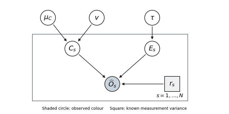
Thus the parent sets are $\boxed{\mathrm{pa}(C_s)=\{{\mu }_C,v\},\mathrm{pa}(E_s)=\{\tau \},\mathrm{pa}(o_s)=\{C_s,E_s,r_s\}}$. Independent hyperparameter prior factors are represented by the three root nodes. With the printed improper priors this is a factorization diagram; it becomes a normalized generative model after proper priors are supplied.

Use the abbreviations in (i). Keeping only terms involving $C_s$ in the joint kernel and completing the square givesConsequently the Gaussian latent-colour update isThese $N$ updates are conditionally independent given the remaining variables. The flat mean prior gives one more normal full conditional:The factorization uses ${\sum }_s(C_s-{\mu }_C{)}^2={\sum }_s(C_s-\overline{C}{)}^2+N({\mu }_C-\overline{C}{)}^2$. Together these are the $N+1$ normal draws in the formal Gibbs sampler.

The terms involving $E_s$ giveCompleting the square produces the truncated normal distributionFor $m=o_s-C_s-r_s/\tau$, its normalized density is $\varphi ((E_s-m)/\sqrt{r_s})/[\sqrt{r_s}\Phi (m/\sqrt{r_s})]$ on $E_s\ge 0$. The exponential prior shifts the untruncated conditional mean downwards before truncation; changing the variance here to the intrinsic variance would be incorrect. These are the other $N$ latent-variable updates of the formal Gibbs sampler.

Keeping the powers and exponentials of $v$ and $\tau$ in the joint kernel gives the two inverse-gamma distributions, using the printed shape–scale convention:Indeed their kernels are $v^{-(N/2+1)}\exp [-{\sum }_s(C_s-{\mu }_C{)}^2/(2v)]$ and ${\tau }^{-(N+1)}\exp [-{\sum }_s{E}_s/\tau ]$. With positive measurement variances and generic continuously drawn latent values, the two scale parameters are positive almost surely. Together with (a),(b), these are all $2N+3$ formal full conditional updates.

There is, however, no joint posterior probability distribution to sample under the stated priors. Integrate out the intrinsic $C_s$ first. For fixed ${\mu }_C,v>0$, the observational marginal density iswhere ${\varphi }_V$ is the centred normal density of variance $V$. Substitute $E=\tau u$. Dominated convergence givesThe convergence is uniform on any compact ${\mu }_C$ interval and any compact positive $v$ interval, since the normal densities are uniformly bounded and continuous there. Hence some such region has $L\ge c>0$ for all sufficiently small $\tau$, andIntegrating over those positive-measure intervals proves that the full normalizing constant is infinite. If all $r_s>0$, the $v\downarrow 0$ boundary also gives a positive marginal likelihood and a divergent $dv/v$ integral at fixed $\tau >0$. Thus $\boxed{\text{the stated joint posterior is improper}}$, even though its generic full conditionals are proper. Apparent stability of a simulated chain cannot establish a nonexistent stationary probability law.

A valid repair that preserves direct sampling is to replace the two log-flat priors by independent proper $v\sim \mathrm{IG}(a_v,b_v)$ and $\tau \sim \mathrm{IG}(a_{\tau },b_{\tau })$, with all four constants positive. The normal and truncated-normal updates remain as above, whileWith positive $r_s$, the flat ${\mu }_C$ prior is then harmless: after integrating it out, the Gaussian measurement likelihood is bounded uniformly over the latent shifts and the scales, and the remaining proper priors integrate to one. A proper prior on ${\mu }_C$ is also possible.

For this repaired model, initialize $v,\tau >0$, $E_s\ge 0$ and finite $C_s,{\mu }_C$. Repeatedly choose one of the $2N+3$ coordinates with fixed positive probabilities and redraw from its full conditional using the latest values. This Random-scan Gibbs sampler preserves the proper target and satisfies detailed balance: for each coordinate, both forward and reverse flows equal the marginal density of the remaining coordinates times the product of the two conditional densities. A systematic full sweep is another invariant scheme, though it need not itself be reversible.

Run several dispersed chains; inspect traces of both scales, ${\mu }_C$, representative latent values and the log posterior. Assess rank-normalized split $\hat{R}$, autocorrelation, and the effective sample size of a Markov chain, and extend runs until relevant Monte Carlo errors are sufficiently small. Scale–latent dependence can cause slow mixing, so diagnostics must include boundary exploration and alternative initializations. Keep post-warmup draws without automatic thinning. These are convergence checks for the repaired posterior; the printed model admits only the formal update algorithm, not a valid posterior-sampling interpretation.