Use the outgoing Green function for the three-dimensional Helmholtz equationLet point out of the obstacle into the exterior. Apply Green second identity to the field and in a large exterior region. Their Sommerfeld radiation conditions make the outer-sphere contribution vanish. The normal on the exterior region's inner boundary is , so the Kirchhoff–Helmholtz representation isThe first integral is the incident source field . Therefore the scattered field is the surface term. Since solves the homogeneous Helmholtz equation within the obstacle, its surface term is zero at exterior observation points; the same representation can be written using only scattered-field traces:The unknown boundary condition determines these traces, but the representation itself does not require choosing that condition.
For large , the outgoing kernel hasThus the surface representation of an obstacle far-field pattern, with , givesConjugating the Herglotz wave function gives . Interchanging the angular and obstacle-surface integrals yields the Herglotz pairing with an obstacle far field:This contains only the scattered-field boundary traces and the Herglotz function, with the outward-obstacle normal convention fixing the sign.
The boundary identity gives a numerical route to shape recovery from a Herglotz boundary identity. First recover an admissible density from measured far-field patterns, enforcing the supplied Herglotz pairing with an obstacle far field for available incident directions:Then evaluate its Herglotz wave function throughout a search region and find a smooth positive radial profile satisfyingThe same must work for every azimuth , expressing the assumed axial symmetry. In practice expand and in basis functions, enforce these equations at collocation points, and minimize the complex residual together with the far-field-data residual. The exclusion of an interior Dirichlet eigenvalue ensures uniqueness of the interior Dirichlet problem for the trial boundary data. Use regularization of an inverse problem to control measurement error and unstable density components; neither uniqueness nor numerical stability follows merely from writing the residual equations.
For rich incident-direction data, the conjugated pairing constraints form an adjoint far-field integral equation for . For only one fixed incidence, the displayed pairing is a single complex scalar constraint and cannot by itself determine an arbitrary density. Additional data or a joint constrained shape fit is then needed; the trace condition supplies the actual geometric information.
Let be the scattering potential supported in . The background Helmholtz equation and its outgoing kernel give the scalar Lippmann-Schwinger equationReplacing the unknown field in the integral by the incident field gives the Born approximation for scalar wave scattering:For the Rytov approximation, work where and set . Dividing the wave equation by the total field and subtracting the incident equation givesNeglect the quadratic gradient term. If , direct differentiation shows , soExpanding the exponential in the potential gives . Thus both approximations have the same first-order field, although exponentiation retains a particular family of higher powers.
For unit plane wave incidence , define the scattering wavevector difference andThe outgoing Green function for the three-dimensional Helmholtz equation givesThe Born far-field pattern is , a Fourier transform sample of the potential. Expanding the far-field Rytov exponential in gives the same leading outgoing term, while the logarithmic representation preserves its accumulated phase and amplitude correction.
Use the leading far-field kernel from the previous part. DefineThen and, because the incident intensity is one,To first order in weak contrast, . Its linearized part is a centered stationary Gaussian random field, with autocorrelation function of a random field . The exponential moment of a Gaussian linear functional therefore gives the usual Gaussian intensity in the first Rytov approximation:Equivalently the exponent is . The second term generally matters because a finite real random medium need not generate a circular complex Gaussian amplitude.
If the full stated potential is retained, it is not Gaussian and has mean . To retain every term through order in the intensity of this first Rytov field, the cumulant expansion instead givesHere ; the raw autocorrelation differs by . The stated remainder uses Gaussian finite-dimensional statistics of , for which odd total moments vanish. This mean term is absent if one first truncates the potential to . Both formulas concern the first Rytov approximation, and exponentiating it does not supply the omitted higher-order scattering corrections.
For admissible data, the Moore–Penrose inverse of an operator selects the minimum-norm least-squares solution:Its domain is . When the equation is consistent it is the solution of orthogonal to the kernel; for inconsistent admissible data it solves the normal equation for a linear inverse problem and projects away the component orthogonal to the range.
Take a singular system of a compact operator satisfying , . The generalized inverse isThe Picard criterion requires the squared coefficients to be summable. For an infinite-rank compact operator, , so even though . Hence is unbounded. Finite-rank compact operators do not have this obstruction. Data failing the Picard condition need not have a least-squares minimizer at all, even when the infimum residual is zero.
A regularization of an inverse problem replaces the unbounded generalized inverse by bounded operators satisfying as on admissible exact data. A spectral regularization method can be writtenwhere for fixed while remains bounded for each fixed . A uniform bound on supplies the usual dominated-convergence argument on exact data.
This defines as the dimensionless damping factor. In the alternative convention calling the entire inverse coefficient the spectral filter, that filter is . For data error bounded by , a sufficient regularization parameter choice also requires ; consistency alone does not control noise.
Minimize the data-misfit functional . For a perturbation , , so its gradient is . Gradient descent gives Landweber iteration:On a singular component, the iteration error is multiplied by , whose modulus is less than one. Starting from zero preserves orthogonality to and makes the exact-data iterates converge to .
For the unit-step formulas and noise bound used below, rescale so that and . Finite iteration count bounds amplification of small singular-value components; the stopping count provides the regularization parameter.
Use early stopping of Landweber iteration. For each finite , the Landweber spectral filter gives a bounded reconstruction operator; as , it approaches the generalized inverse on exact admissible data. Taking , a sufficient rule for a convergent regularization of an inverse problem isor equivalently and . For example, satisfies both in the normalized problem. The first condition removes exact-data bias; the second prevents arbitrarily small measurement errors from being amplified by excessive iteration.
Add and subtract the exact-data iterate. The noise-bias decomposition for linear regularization givesso the supplied Landweber noise amplification bound yieldsWith unit step and zero initial iterate, the exact-data error is . Its squared norm isby the dominated convergence theorem. Stopping with but therefore makes both errors vanish.
On each left singular vector , use and . The finite geometric series givesThus with , the dimensionless Landweber spectral filter isThe full inverse-coefficient convention instead uses . With general step , replace inside the power by .
In the normalized problem, , so the inverse coefficient is at most . This verifies directly why finite iteration is stable and why admitting progressively smaller singular values eventually amplifies noise.
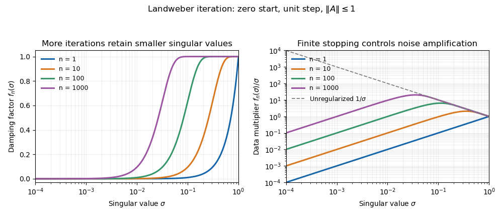
Landweber filters and progressive noise amplification
. More iterations admit smaller singular-value components. The damping factor tends toward one, while the coefficient applied to measured data approaches the unstable reciprocal singular value. Details.
Articles by others on the same topic
There are currently no matching articles.