For admissible data, the Moore–Penrose inverse of an operator selects the minimum-norm least-squares solution:Its domain is . When the equation is consistent it is the solution of orthogonal to the kernel; for inconsistent admissible data it solves the normal equation for a linear inverse problem and projects away the component orthogonal to the range.
Take a singular system of a compact operator satisfying , . The generalized inverse isThe Picard criterion requires the squared coefficients to be summable. For an infinite-rank compact operator, , so even though . Hence is unbounded. Finite-rank compact operators do not have this obstruction. Data failing the Picard condition need not have a least-squares minimizer at all, even when the infimum residual is zero.
A regularization of an inverse problem replaces the unbounded generalized inverse by bounded operators satisfying as on admissible exact data. A spectral regularization method can be writtenwhere for fixed while remains bounded for each fixed . A uniform bound on supplies the usual dominated-convergence argument on exact data.
This defines as the dimensionless damping factor. In the alternative convention calling the entire inverse coefficient the spectral filter, that filter is . For data error bounded by , a sufficient regularization parameter choice also requires ; consistency alone does not control noise.
Minimize the data-misfit functional . For a perturbation , , so its gradient is . Gradient descent gives Landweber iteration:On a singular component, the iteration error is multiplied by , whose modulus is less than one. Starting from zero preserves orthogonality to and makes the exact-data iterates converge to .
For the unit-step formulas and noise bound used below, rescale so that and . Finite iteration count bounds amplification of small singular-value components; the stopping count provides the regularization parameter.
Use early stopping of Landweber iteration. For each finite , the Landweber spectral filter gives a bounded reconstruction operator; as , it approaches the generalized inverse on exact admissible data. Taking , a sufficient rule for a convergent regularization of an inverse problem isor equivalently and . For example, satisfies both in the normalized problem. The first condition removes exact-data bias; the second prevents arbitrarily small measurement errors from being amplified by excessive iteration.
Add and subtract the exact-data iterate. The noise-bias decomposition for linear regularization givesso the supplied Landweber noise amplification bound yieldsWith unit step and zero initial iterate, the exact-data error is . Its squared norm isby the dominated convergence theorem. Stopping with but therefore makes both errors vanish.
On each left singular vector , use and . The finite geometric series givesThus with , the dimensionless Landweber spectral filter isThe full inverse-coefficient convention instead uses . With general step , replace inside the power by .
In the normalized problem, , so the inverse coefficient is at most . This verifies directly why finite iteration is stable and why admitting progressively smaller singular values eventually amplifies noise.
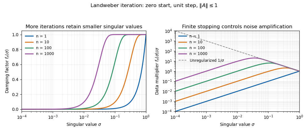
Landweber filters and progressive noise amplification
. More iterations admit smaller singular-value components. The damping factor tends toward one, while the coefficient applied to measured data approaches the unstable reciprocal singular value. Details.
Articles by others on the same topic
There are currently no matching articles.