Past exam of the mathematics course of the year 1 of the natural sciences course of the University of Cambridge / 2008 / Paper 1 / 15

For the binomial distribution and $T\ge 1$, the identity $s\left(\genfrac{}{}{0ex}{}{T}{s}\right)=T\left(\genfrac{}{}{0ex}{}{T-1}{s-1}\right)$ gives the expectationThe final sum is one by the binomial theorem. For $T=0$ the variable is identically zero, so the same answer holds:

For an integrable discrete random variable, its expectation and variance are $\mu ={\sum }_{n\in \mathbb{Z}}n{p}_n$ and ${\sum }_{n\in \mathbb{Z}}(n-\mu {)}^2{p}_n$, respectively. The first formula requires $\sum |n|p_n<\infty$ for a finite ordinary mean; the variance may be infinite. A probability density function gives $P(\alpha <Y<\beta )={\int }_{\alpha }^{\beta }f(y)dy$.

Conditioning on $X$ and using independence givesThe interchange is justified by Tonelli's theorem, since all integrands are nonnegative. Consequently $Z$ has an absolutely continuous distribution, withIts integral is ${\sum }_n{p}_n=1$. This is the convolution of independent random variables, specifically a Gaussian smoothing of an integer-valued distribution for the given normal density. The specified weights are normalized because $2(3/{\pi }^2){\sum }_{n\ge 1}{n}^{-2}=1$.

The density is the symmetric sumFor small $\sigma$, the normal distributions are narrow and well separated, giving peaks near each nonzero integer. The largest two peaks lie near $-1$ and $1$; those near $\pm 2$ have approximately one quarter of their height, and the envelope falls as $1/n^2$. There is no component centered at zero, and the density there is exponentially small. The left panel shows the resulting smooth comb.

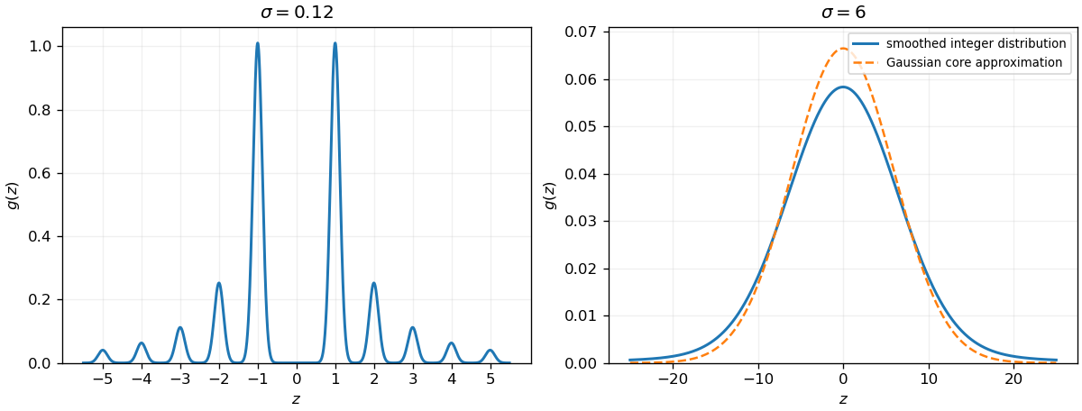
For large $\sigma$, neighboring peaks overlap and the density has a broad, smooth, symmetric central hump, approximately $(\sqrt{2\pi }\sigma {)}^{-1}{e}^{-z^2/(2{\sigma }^2)}$ on the scale $z=O(\sigma )$. A precise central-profile statement follows fromfor each fixed $t$, $X/\sigma \to 0$ almost surely and the integrand is bounded, so dominated convergence applies. The right panel of the preceding figure shows this Gaussian-looking core.

This approximation does not remove the heavy-tailed distribution. Here $\mathbb{E}|X|=(6/{\pi }^2){\sum }_{n\ge 1}1/n=\infty$, so the symmetric distribution has no ordinary mean and no finite variance. Adding the independent Gaussian, which has finite absolute moments, leaves these conclusions unchanged. In particular a central Gaussian sketch cannot justify assigning variance ${\sigma }^2$ to $Z$.