The angle-subtraction identity gives . Thus , so . Keeping the two values in the specified interval gives
The chain rule gives
Use the change of variables , . ThenDifferentiating verifies this antiderivative on the whole real line.
The point on the parabola is . Implicit differentiation gives , so the tangent line has slope one there. Its perpendicular normal line to a plane curve therefore has slope . The required line is
Write . The graph is a translated hyperbola, with vertical asymptote and horizontal asymptote . It passes through , lies below for and above it for , and has derivative on each component of its domain. The left panel below shows both branches.
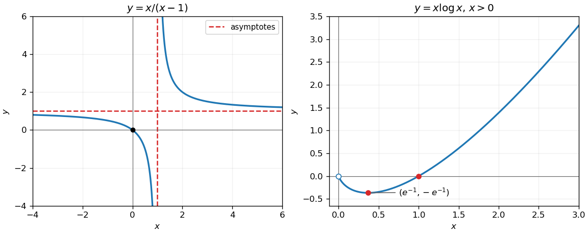
The domain is , and from below as . Its derivative is , so it decreases up to and then increases, with its unique global minimum at . It crosses the horizontal axis at and tends to as . Its second derivative is , so it is strictly convex. The right panel of the preceding figure shows these features; zero is an excluded endpoint with a finite limiting value, rather than a vertical asymptote.
Evaluate the absolute values on the three intervals separated by one and two:The strict inequality therefore holds precisely for
Let be the top vertex, the center, and the two other points on the circle. The diameter bisects the angle at , so the two right triangles obtained by drawing the diameter to the opposite point show that have coordinates when and . The chord cuts off a lower circular segment of central angle . The triangle has area , while the segment has area , by subtracting the central triangle from its circular sector. Adding giveswith measured in radians. This is the unit-radius case of the area enclosed by two chords and a circular arc.
The two finite summations cancel term by term after shifting the index. Only the final positive term remains:This is a telescoping sum.
Since , the vector is perpendicular to :It follows that . If , then ; if , then . Thus is the orthogonal projection matrix onto : it removes exactly the component normal to the plane.
For the equally inclined plane choose . Reversing its sign gives the same plane; other sign choices give equivalent reflections of the coordinate axes. One suitable orthonormal basis of this plane isTheir dot products with vanish, their lengths are one, and their mutual dot product is zero. The equal first two components of give its equal inclinations to . Because is already in the projection plane, . The coordinates of the projected point are thereforeFor a circle of radius centered at the origin in , its equation becomes . This is an ellipse with semiaxes and . Translating the original center only translates its orthogonal projection, so the result applies to every circle in that plane. ConsequentlyThe general reason is the orthogonal projection of a circle between planes: the direction common to the planes retains its length, while the perpendicular direction is shortened by the cosine of their angle.
The relation rearranges to , so the diagonals and have the same midpoint. Equivalently and : each pair of opposite sides has the same displacement vector. Thus the given quadrilateral is a parallelogram. The identities also describe degenerate configurations if coincident or collinear vertices are allowed.
Multiply numerator and denominator by the complex conjugate of . For this givesThus its real part and imaginary part are respectively
Multiplying by gives . The sixth roots of unity do not solve the original equation, since substituting either gives three. The other four do, because the extra factor is nonzero. HenceTheir real parts are and their imaginary parts are , giving the four corners in the left Argand diagram below.
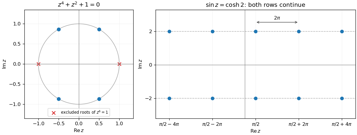
Writing and comparing real parts and imaginary parts gives and . A real solution is impossible since . Thus , and positivity forces . Consequently and , givingThe right Argand diagram in the preceding figure shows representative points on the lines ; each row continues with spacing .
For , the geometric series gives . Its uniform convergence on every closed interval strictly inside permits termwise integration from zero to . ThereforeSubtracting cancels every even power and doubles every odd power, giving the Taylor series
Use the binomial series and exponential Maclaurin series:The Cauchy product isAdding cancels the first three powers. Hence the first nonzero term is
Put . The rational factor has Taylor expansion . Multiplication by the logarithmic power series makes the coefficients of equal to and . Setting both to zero gives and , henceThe coefficient of is . Thus the resulting expansion begins .
The domain of integration is , . Reversing the order in the double integral and then putting givesTherefore
The base is the disk , on which . The vertical thickness is . Using the symmetry of the disk about , or integrating with , givesFor the curved cylindrical surface use , , with and . The area element is . Its surface area is thereforeThe sloping planar faces are excluded from this curved surface area.
For the binomial distribution and , the identity gives the expectationThe final sum is one by the binomial theorem. For the variable is identically zero, so the same answer holds:
For an integrable discrete random variable, its expectation and variance are and , respectively. The first formula requires for a finite ordinary mean; the variance may be infinite. A probability density function gives .
Conditioning on and using independence givesThe interchange is justified by Tonelli's theorem, since all integrands are nonnegative. Consequently has an absolutely continuous distribution, withIts integral is . This is the convolution of independent random variables, specifically a Gaussian smoothing of an integer-valued distribution for the given normal density. The specified weights are normalized because .
The density is the symmetric sumFor small , the normal distributions are narrow and well separated, giving peaks near each nonzero integer. The largest two peaks lie near and ; those near have approximately one quarter of their height, and the envelope falls as . There is no component centered at zero, and the density there is exponentially small. The left panel shows the resulting smooth comb.
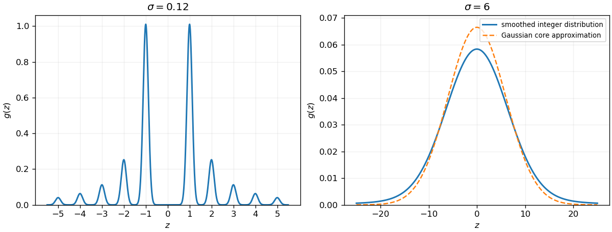


For large , neighboring peaks overlap and the density has a broad, smooth, symmetric central hump, approximately on the scale . A precise central-profile statement follows fromfor each fixed , almost surely and the integrand is bounded, so dominated convergence applies. The right panel of the preceding figure shows this Gaussian-looking core.
This approximation does not remove the heavy-tailed distribution. Here , so the symmetric distribution has no ordinary mean and no finite variance. Adding the independent Gaussian, which has finite absolute moments, leaves these conclusions unchanged. In particular a central Gaussian sketch cannot justify assigning variance to .
The separable differential equation gives . Thus on , and the initial value gives . HenceThe initial-value branch cannot cross its singularity at zero.
On an interval avoiding zero put . A real solution requires , and the principal square root is . The homogeneous first-order differential equation reduces toWhere , separation of variables gives . Thus the nonconstant pieces arerestricted to intervals where the cosine of the phase is nonnegative. This sign condition is essential when substituting back into the original square root.
There are also the solutions and . They can join the nonconstant pieces with a continuous first derivative, because the transformed rate vanishes but is not Lipschitz continuous at . For example, on the positive axis every givesThe sticking solutions of a bounded square-root differential equation describe the same joining mechanism on either half-axis after using the increasing variable .
Near the initial point, division by gives . An integrating factor is , andThus , and givesAlthough division by was local, direct substitution verifies this smooth solution in the original equation for every real , including the zeros of .
Set , so . The equation becomes . For its integrating factor is , givingThe initial value is , forcing . HenceSubstitution into the original equation verifies this answer throughout , including where the divided linear equation was singular. Its maximal connected interval through the initial point is .
The zero set consists of the three lines , and . Their pairwise intersections areThe bounded triangle has and . Its edges and interior contours are shown below.
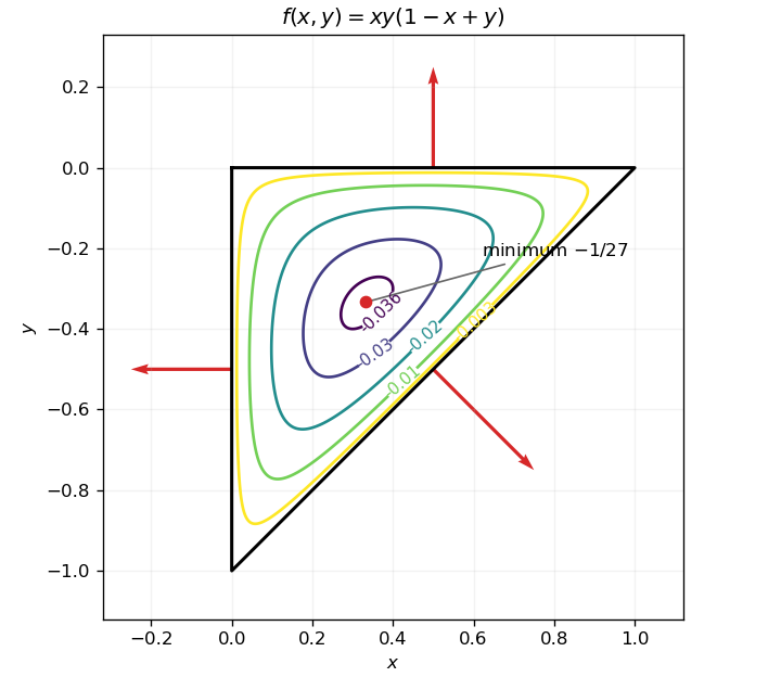
Negative contours inside the zero triangle, with outward boundary gradients and the interior minimum
. Details. 
The gradient is . At the three specified points it is respectivelyEach vector is perpendicular to its straight boundary edge and points out of the triangle, where increases from its negative interior values. The arrows in the preceding figure mark these directions.
Inside the triangle, both and are nonzero. Thus reduces to and , whose unique solution is . At that pointThe Hessian matrix has positive eigenvalues and , so this is a strict local minimum. It is also the minimum on the closed triangle: on the boundary, inside, and there is no other interior stationary point. Therefore
The interior values satisfy away from the minimum. The contours are closed curves surrounding , approximately ellipses near that point, and approach the three edges as the level tends to zero. To see their shape globally, put , , . These are positive inside and satisfy , while . Since is strictly concave, its nonempty superlevel sets are convex and surround the unique maximum of . Thus the negative contours nest without additional components, as in the figure.
The gradient is . Its second component vanishes only if or . The latter gives the impossible first-component equation . With , the first component gives or . The Hessian matrix isAt it has eigenvalues , giving a saddle point. At its eigenvalues are , giving a strict local minimum, of value . These are all real stationary points. The minimum is local: for example as .
Articles were limited to the first 100 out of 249 total.
Articles by others on the same topic
There are currently no matching articles.