Disperse a very small amount of the dry powder in a clean volatile solvent compatible with aluminium oxide, use brief gentle sonication to separate loose agglomerates, and place a dilute drop on a holey carbon-coated transmission electron microscopy grid. Wick away excess liquid and dry thoroughly. Look first at low magnification and select isolated particles or thin edges over holes, rather than an electron-opaque pile. Record a solvent-only grid to identify contamination and compare several independently prepared areas.
This is quick and preserves individual particles without mechanical thinning. However, spray pyrolysis can make hollow or porous particles that may fracture during sonication; sedimentation and drying can select sizes and aggregate particles. aluminium oxide is insulating, so charging or beam-induced changes can complicate images, and the carbon support can overlap weak contrast. Vary dose and dwell time to test stability. A projected image of one selected thin particle is not an unbiased three-dimensional size or porosity distribution of the whole powder.
This is a conventional transmitted-beam bright-field transmission electron microscopy image containing high-resolution electron phase contrast and visible lattice fringes, rather than an element-specific chemical map. Relative to the scale bar, the smaller particle has an outer projected diameter of roughly . It is approximately rounded and contains a denser outer rim with several lighter internal regions separated by material. A porous or internally hollow particle is a plausible morphological interpretation; the image is not a simple featureless solid sphere.
Greater projected thickness generally removes more intensity from the transmitted beam, producing darker mass–thickness contrast. Different crystallite orientations also scatter intensity differently and give diffraction contrast. Local lattice fringes reveal crystalline material and changes of fringe orientation indicate more than one coherent domain. Bright/dark edge fringes also contain defocus-dependent Fresnel contrast; their width is not a direct shell-thickness measurement. Neither an exact alumina polymorph nor three-dimensional closed porosity can be uniquely established from this projection alone. Use calibrated fringe spacings and electron diffraction for phase identification, tilt-series imaging for void geometry, and a through-focus or dose series to test contrast artefacts.
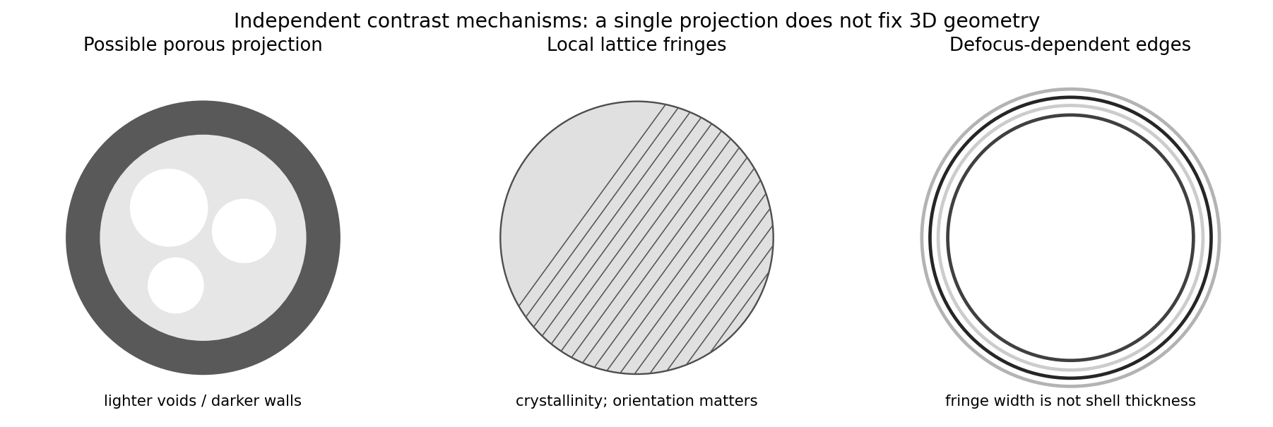
Original generic schematic separating projected porosity, crystallite orientation and edge-contrast interpretations
. Details. 
For a weak phase object, the contrast transfer function gives the signed transfer of an object's spatial Fourier components into intensity contrast. In a common convention,where is a cyclic spatial frequency, the defocus, the spherical aberration coefficient, and a coherence envelope. A zero suppresses that frequency; crossing a zero reverses contrast. The overall sign depends on the image convention, but the zeros do not. Single-image division by cannot recover information exactly at its zeros. The microscope manufacturer's discussion explicitly connects the first zero with interpretable resolution and the higher-frequency sign changes.[ref]
Phase-contrast transfer function, PCTF by JEOL. glossary, first-zero and envelope-function discussion
The plotted first nontrivial zero is at approximately . Hence the smallest spacing in the first uninterrupted contrast band is about . This axis is cycles per length, not an angular wave number requiring a factor of . Smaller spacings can contribute in later bands, but their contrast has reversed and requires appropriate interpretation or multiple-defocus reconstruction.
There is a verified inconsistency in the printed data: the original PDF says , whereas the relativistic de Broglie wavelength at is approximately :Use consistent length units, , and distinguish literal arithmetic from a physically consistent estimate. The familiar approximate Scherzer defocus is , or about with . Slightly different optimum-phase conventions use in place of , giving about ; both are underfocus by a few tens of nanometres. The manufacturer's tabulated values confirm that scale.[ref]
Scherzer focus by JEOL. glossary, underfocus convention and accelerating-voltage/spherical-aberration table
Using the question's additional numerical relation exactly as supplied, with , givesFor the physically appropriate rounded wavelength this is . The CTF itself gives an independent check: its first nonzero zero satisfies , so implies . The plotted condition is therefore a little less underfocused than the usual Scherzer setting and has a first-zero spacing near . The nominal and approximate optimization formula should not be treated as exactly reproducing every plotted parameter.
If the printed is retained literally, the approximate Scherzer formula instead gives , the supplied relation gives , and the plotted first zero requires . These do not describe a consistent microscope. The physically consistent comparison is approximately to optimum underfocus versus from the plot; the wavelength correction is explicit.
Articles by others on the same topic
There are currently no matching articles.