Original archive: Cambridge FOI 2024/50 released ZIP. The original is the member
NanoMPhil Paper 1 2019.pdf, physical pages 1–15.The repeated, similarly oriented rounded triangular outlines in panel (a) are characteristic of AFM tip convolution: a narrow raised object can image the shape of a blunt or contaminated AFM probe, rather than reveal its own lateral shape. A finite tip radius broadens lateral dimensions. Replace or clean the AFM probe, check it on an independently characterized sharp-feature standard, and repeat at low load; agreement after a tip change is stronger evidence than a visually pleasing image. Image processing cannot uniquely recover unmeasured sidewalls or prove that every particle with a similar outline is an artefact.
Panel (b) contains horizontal streaks associated with steep features. The natural instrumental diagnosis is AFM feedback artefact: the height controller does not track a rapid change faithfully, or rings after it. Reduce the scan speed and adjust proportional/integral gains below the oscillation threshold. Compare trace and retrace and rotate the fast-scan direction: a streak following the scan rather than the specimen is instrumental. Loose contamination can also produce scan-line streaks, so clean or change the AFM probe if tuning does not remove them. Tip-shape broadening in (a), and scan-direction tracking/streaking in (b), are the principal diagnoses; the images alone do not uniquely establish every underlying cause.
piezoelectric scanner creep is the continued slow displacement after a step in scanner drive, even when the commanded voltage has stopped changing. The scanner's strain continues to relax, and the motion can resemble a slowly decaying, approximately logarithmic drift. After changing scan size, position or offset, early lines can therefore have stretched or compressed coordinates. Allow settling, avoid large abrupt moves, use a position-sensor closed-loop control system, and compare repeated images. This time-dependent response differs from the direction-dependent piezoelectric hysteresis and from ordinary thermal drift.
A steady-current image is not supported by the electrical connection drawn. tunnelling atomic force microscopy requires a conducting AFM probe, an applied bias voltage and a continuous return path from the contacted region to the current amplifier. graphene is conducting, but a flake on insulating glass is not electrically grounded merely because the other side or edge of the glass is earthed. Charging transients or displacement current are not its steady conductivity. Add a metal contact actually touching the graphene before using its current contrast; ordinary force-based surface topography can still be recorded without that contact. The manufacturer's nanostructure measurements explicitly distinguish objects connected to conducting pads from unconnected particles on the same insulating substrate.[ref]
Simultaneous Electrical and Mechanical Property Mapping at the Nanoscale with PeakForce TUNA by Bruker. application note 132, Figure 11 and accompanying discussion of electrical connection
quantitative nanomechanical mapping can image the flake without an electrical return path. Repeated AFM force curves provide surface topography, adhesion and deformation or effective elastic modulus channels. The step and differences in tip–surface interaction can distinguish graphene from glass. For an atomically thin supported sheet the contact response is strongly substrate dependent, so fitting a three-dimensional half-space contact model does not directly measure the intrinsic in-plane Young's modulus of free graphene. Calibrate the cantilever spring constant, deflection sensitivity and tip radius, use small loads, and compare bare substrate. The manufacturer's description specifies the force-curve origin of the mechanical channels.[ref]
Simultaneous Electrical and Mechanical Property Mapping at the Nanoscale with PeakForce TUNA by Bruker. application note 132, Quantitative Mechanical Property Mapping
friction force microscopy is suitable. Contact scanning twists the AFM cantilever; the lateral photodetector difference measures friction and can distinguish the supported graphene and glass even if their heights are close. Acquire both trace and retrace and use half their lateral-signal difference to suppress slope-induced cross-talk. Keep the normal load low enough to avoid dragging or damaging the flake, control humidity and contamination, and calibrate torsional sensitivity if a quantitative coefficient of friction is required. An electrical connection is unnecessary.
Conventional semiconductor scanning capacitance microscopy is not a reliable dopant-contrast image of this specimen as drawn. Its usual signal relies on a tip–insulator–semiconductor capacitance whose depletion region changes under AC bias. An isolated conducting graphene sheet on thick insulating glass provides neither that conventional depletion geometry nor a controlled charge reservoir; simply earthing glass does not supply one. Capacitive or electrostatic contrast may be detectable with a suitably designed back electrode, a contacted flake and an appropriate capacitance-sensitive instrument, but that is an additional electrical device specification. Force-based surface topography remains possible independently of the specialized capacitance channel.
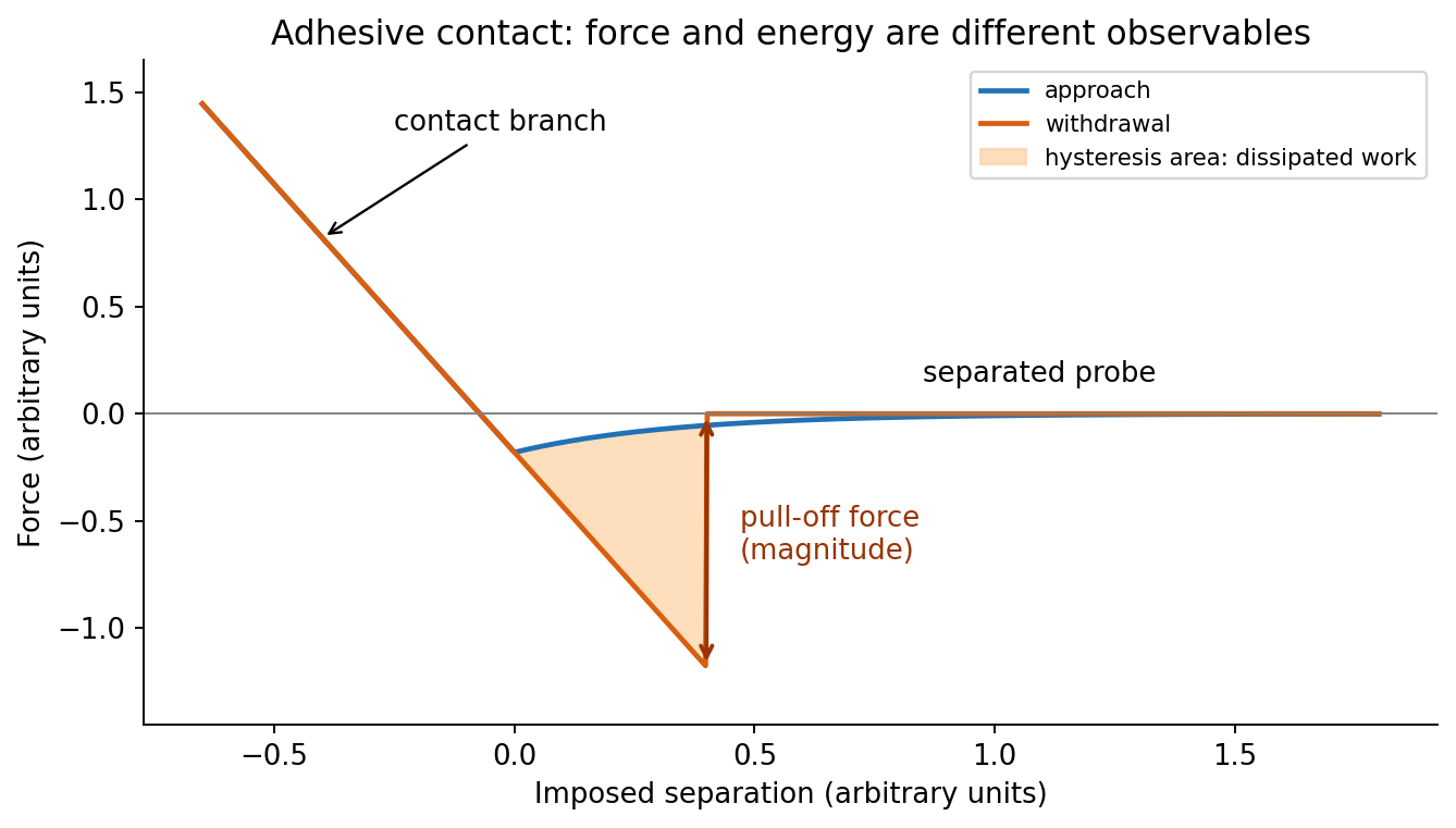
At position (1), the AFM probe is far from the surface, with approximately zero force. At (2), attractive interactions bend the AFM cantilever toward the surface; when the attractive force gradient exceeds the cantilever spring constant, the equilibrium becomes unstable and jump-to-contact occurs. Position (3) is on the mechanical-contact branch: changes in imposed height largely bend the AFM cantilever and, for a compliant specimen, indent the sample. This branch can include compressive contact and adhesive contact under tension; contact does not itself imply a positive force at every point. At (4), during withdrawal the tip remains attached and pulls the AFM cantilever downward until the pull-off force is reached and it detaches. Approach and retraction follow different paths because adhesion creates a hysteretic contact. The numbered points identify stages on the source curve, not four extra question parts.
In quantitative nanomechanical mapping, the operational adhesion is the magnitude of the most attractive force immediately before detachment on a calibrated retraction curve:Here is the cantilever spring constant and its deflection after baseline subtraction. The area between approach and retraction relates to dissipated work, whereas the minimum force is a force, not an energy. Chemical attraction, Van der Waals forces and ambient-water capillary bridges can all contribute. Match loading rate and peak load, calibrate deflection sensitivity and , compare clean reference surfaces, and control humidity; otherwise different maps may reflect different tips or capillary conditions rather than different specimens.

Three suitable approaches give complementary contrast. tapping-mode atomic force microscopy supplies surface topography and an oscillation-phase image. It reduces lateral drag and is often effective for soft block copolymer domains. Its phase contrast depends on elastic response, adhesion, dissipation and operating setpoint together: a bright phase domain is not automatically the stiffer polymer. Check contrast as amplitude and setpoint change and use a known reference.
quantitative nanomechanical mapping fits the repulsive portions of many AFM force curves and separately maps effective elastic modulus, adhesion and deformation. It directly addresses the stiffness difference and limits maximum force. Its quantitative result depends on tip radius, force calibration, contact model, loading rate and film thickness; domains narrower than the contact footprint are mixed and the substrate can dominate a thin film. Use small indentation, substrate controls and a suitable viscoelastic interpretation.
friction force microscopy can reveal domains with different frictional and adhesive response, using torsional deflection during contact scans. It is simple and sensitive to surface chemistry, but continuous shear may deform or displace soft domains, and slope/topography can contaminate the lateral signal. Acquire trace–retrace pairs at several low normal loads and check reproducibility. Use a mechanical-modulus map to test the stiffness assignment; phase or friction contrast alone does not uniquely identify stiffness or chemical composition.
For a positive photoresist, let be the largest exposure preserving the initial film thickness and the clearing dose. The photoresist contrast is . An aerial image can clear its maxima while retaining its minima only ifThus and for the lower- and higher-contrast materials. Reading those levels on the supplied modulation transfer function gives maximum normalized spatial frequencies approximately and , respectively. The stated partial coherence is already represented by that curve; do not multiply the read frequencies by another coherence factor.
The unambiguous pattern dimensions are full pitch and equal line/space width , where is the read normalized frequency. To convert the paper's Rayleigh-frequency label into lengths, explicitly use the circular-pupil Rayleigh criterion and . With the ArF vacuum wavelength and the stated numerical aperture, , givingThe higher-contrast material resolves a line/space feature about two-thirds as wide. The pitch and half-pitch distinction matters: the point-separation Rayleigh criterion is not itself an equal-line/space width. If a course defines as an optical cutoff rather than , use that specified frequency in ; the normalized graph readings and their ratio are unchanged. No absolute clearing dose is provided.
On a graph of normalized remaining thickness against , both positive photoresist curves remain near unity below and fall to zero by . Their transition widths are : decades for the lower-contrast material and decades for the higher-contrast material. The latter therefore has a much steeper transition. The curves can be aligned at a common illustrative clearing dose; their absolute horizontal placement cannot be inferred from photoresist contrast alone.
The higher-contrast material distinguishes bright and dark regions even when diffraction has reduced their intensity modulation. The lower-contrast material requires a much stronger aerial-image modulation and loses small features earlier. Finite resist thickness, standing waves, acid diffusion, development conditions and photon statistics can limit actual performance beyond this threshold model.
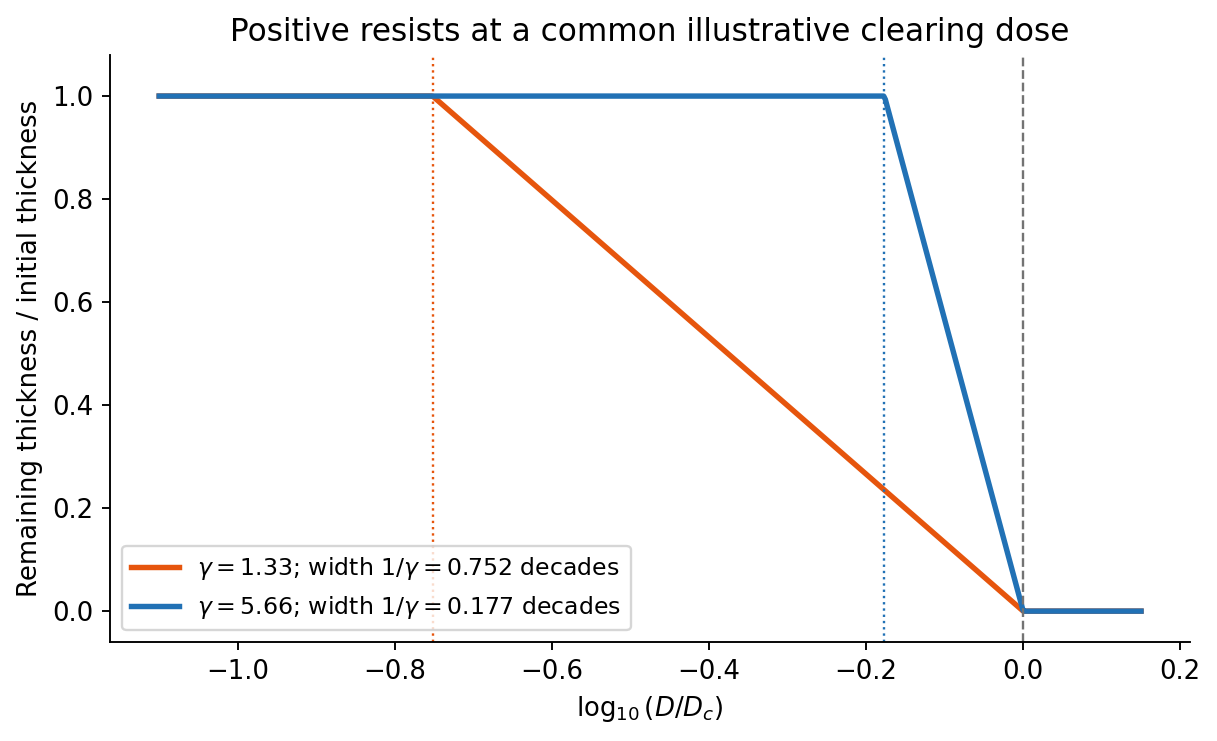
Original normalized positive-resist contrast curves illustrating transition widths, with no assumed absolute sensitivity
. Details. 
Solve the stated depth of focus relation before substituting into the resolution expression:This uses the supplied empirical and unchanged and interprets as the minimum line or space width of an equal-line/space square grating. Under that convention its pitch is . Other pattern shapes or a different definition of the quoted depth of focus would require different process factors.
An immersion liquid increases numerical aperture through , if the optics can use the same ray angle inside a transparent, chemically compatible liquid of refractive index . With unchanged and vacuum wavelength, the width scales as at fixed angle. If the two empirical formulae printed in the question are used literally with fixed , they give .
For a physical axial displacement inside the medium, however, the familiar paraxial defocus range contains an additional index factor: . That convention gives at fixed ray angle, or an approximately -fold larger depth of focus at fixed and resolution. Thus immersion can improve lateral resolution, while its focus benefit depends on what is held fixed and on the axial-focus convention. It cannot improve resolution merely by inserting into while ignoring optical redesign, absorption or resist compatibility. No liquid index is supplied for a numerical prediction.
First, use a phase-shift mask: neighbouring openings transmit appropriately phased light, increasing the intensity slope and improving separation of neighbouring bright regions. The benefit is pattern dependent and phase conflicts or mask defects must be controlled. Second, use off-axis illumination matched to the grating orientation, so useful diffracted orders fall inside the projection pupil and contribute interference contrast at smaller pitch. Check orientation dependence and the reduced process window; it does not enlarge the geometrical pupil.
Third, use optical proximity correction and subresolution assist features to compensate the pattern-dependent aerial-image distortion at edges and corners. Verify the printed critical dimensions using a focus–exposure matrix and scanning electron microscopy. These are three adaptations of the existing exposure process that lower effective ; none promises arbitrary subwavelength structure. A thinner, higher-contrast photoresist and an antireflection underlayer can further improve pattern transfer, but do not change the wavelength.
charge stabilization of colloids supplies repulsion when like-charged surfaces and their electric double layers approach. steric stabilization uses attached or adsorbed molecular layers whose overlap costs conformational and osmotic free energy. Combining both gives electrosteric stabilization; a solvated coating must remain attached and well solvated. A viscous medium slows encounters but does not by itself create an equilibrium repulsive barrier.
DLVO theory adds screened electrostatic repulsion to Van der Waals force. A representative close-gap form isfor equal spheres of radius , with Hamaker constant and inverse Debye–Hückel screening length . The formula is schematic near molecular contact, where hydration, surface roughness and finite ion size matter. A repulsive barrier many high produces kinetic stability even if the primary attractive minimum is deeper than the dispersed state. Entry into that primary minimum generally gives strongly bound aggregation; a shallow secondary minimum can give reversible flocculation.
Adding electrolyte increases , shortens the repulsion and can remove the barrier, enabling fast diffusion-limited aggregation. The critical coagulation concentration is the approximate salt concentration at which this rapid-coagulation regime begins under specified conditions. It is not a universal property of the salt alone. Test the prediction using time-resolved dynamic light scattering or turbidity at controlled particle concentration, pH and temperature; check that added ions do not specifically adsorb or change the surface chemistry.
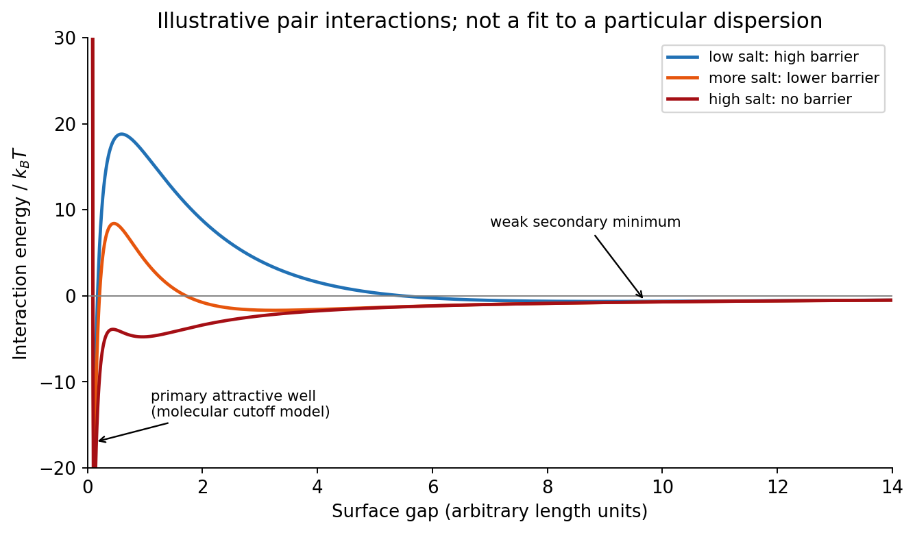
Original schematic DLVO interaction curves showing a stabilizing barrier, secondary minimum and barrier loss on salt addition
. Details. 
In the high-surface-potential Schulze-Hardy rule, the critical coagulation concentration scales approximately as with the counterion valence. HenceThe more highly charged counterion therefore requires about eleven times less concentration in this idealized estimate. This assumes the cations are the counterions of a negatively charged surface, the surface-potential regime is appropriate, and the only changing mechanism is electrostatic stabilization. Specific adsorption and hydrolysis of aluminium ions can invalidate this scaling; matching ionic strengths instead is not the same prediction.
The more negative standard reduction potential identifies iron as the species more readily oxidized. Combining with gives the spontaneous standard galvanic cell reactionThe electron balance is two per reaction, and the activities of the pure metals are unity.
For a galvanic cell, subtract the standard anode reduction potential from the standard cathode reduction potential:A reduction potential is not multiplied by the number of transferred electrons.
Iron is the negative anode and tin is the positive cathode of this spontaneous galvanic cell. electrons travel through the external circuit from iron to tin. An intact tin coating protects iron mainly by physically excluding the corrosive medium. If a defect exposes iron while the metals remain electrically connected, tin is not a sacrificial coating: the exposed iron can become the anodic corrosion site. A small exposed iron area coupled to a large cathodic tin area can be especially damaging; this distinction follows from the electrode-potential order rather than the appearance of the coating.
With , the standard reaction Gibbs free energy and dimensionless equilibrium constant areFor the reaction as written, , and the Nernst equation gives . Consequently zero cell potential requires under the specified unit-activity-coefficient assumption. Reversing that ratio reverses the conclusion. This mathematical ratio does not by itself guarantee experimentally attainable concentrations without precipitation or other chemistry.
A Ragone plot has specific energy on its horizontal logarithmic axis and specific power on its vertical logarithmic axis, normally in and . The comparison must use the same mass convention: complete devices cannot fairly be compared with electrode-active-material values. At approximately constant delivered power, the discharge time isThus constant-time lines slope upward on the log–log plot. Ordinary capacitors lie toward high power and low energy; batteries toward higher energy and lower power; supercapacitors bridge the two. Technology and operating limits produce overlapping regions, not universal sharp boxes.
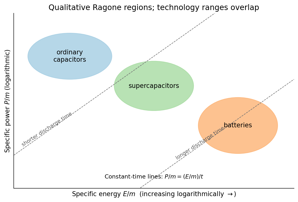
Original qualitative Ragone comparison with logarithmic axes and representative constant-discharge-time lines
. Details. 
An ordinary capacitor stores energy by separating charge across a dielectric: and . Electronic charge redistribution is rapid, giving high specific power, but the dielectric breakdown field and modest capacitance limit specific energy. Series resistance limits pulse power and produces heating; a large nominal capacitance does not remove those losses.
A supercapacitor has a much larger interfacial area and nanometre-scale charge separation. An electric double-layer capacitor stores charge without a bulk redox transformation; pseudocapacitance adds sufficiently fast surface or near-surface redox storage. ion motion in pores, electrolyte stability and series resistance constrain its response. Its specific energy usually exceeds an ordinary capacitor's while high specific power and cycling durability remain possible.
An electric battery stores chemical free energy through coupled electrode oxidation-reduction reactions. It can store substantial energy per mass, but charge transfer, ionic transport, diffusion and heat removal constrain rapid discharge. The terminal voltage and accessible capacity depend on discharge rate and state of charge. Accordingly the plotted order follows the storage and transport mechanisms; it is not a claim that every battery has less power than every supercapacitor.
Disperse a very small amount of the dry powder in a clean volatile solvent compatible with aluminium oxide, use brief gentle sonication to separate loose agglomerates, and place a dilute drop on a holey carbon-coated transmission electron microscopy grid. Wick away excess liquid and dry thoroughly. Look first at low magnification and select isolated particles or thin edges over holes, rather than an electron-opaque pile. Record a solvent-only grid to identify contamination and compare several independently prepared areas.
This is quick and preserves individual particles without mechanical thinning. However, spray pyrolysis can make hollow or porous particles that may fracture during sonication; sedimentation and drying can select sizes and aggregate particles. aluminium oxide is insulating, so charging or beam-induced changes can complicate images, and the carbon support can overlap weak contrast. Vary dose and dwell time to test stability. A projected image of one selected thin particle is not an unbiased three-dimensional size or porosity distribution of the whole powder.
This is a conventional transmitted-beam bright-field transmission electron microscopy image containing high-resolution electron phase contrast and visible lattice fringes, rather than an element-specific chemical map. Relative to the scale bar, the smaller particle has an outer projected diameter of roughly . It is approximately rounded and contains a denser outer rim with several lighter internal regions separated by material. A porous or internally hollow particle is a plausible morphological interpretation; the image is not a simple featureless solid sphere.
Greater projected thickness generally removes more intensity from the transmitted beam, producing darker mass–thickness contrast. Different crystallite orientations also scatter intensity differently and give diffraction contrast. Local lattice fringes reveal crystalline material and changes of fringe orientation indicate more than one coherent domain. Bright/dark edge fringes also contain defocus-dependent Fresnel contrast; their width is not a direct shell-thickness measurement. Neither an exact alumina polymorph nor three-dimensional closed porosity can be uniquely established from this projection alone. Use calibrated fringe spacings and electron diffraction for phase identification, tilt-series imaging for void geometry, and a through-focus or dose series to test contrast artefacts.
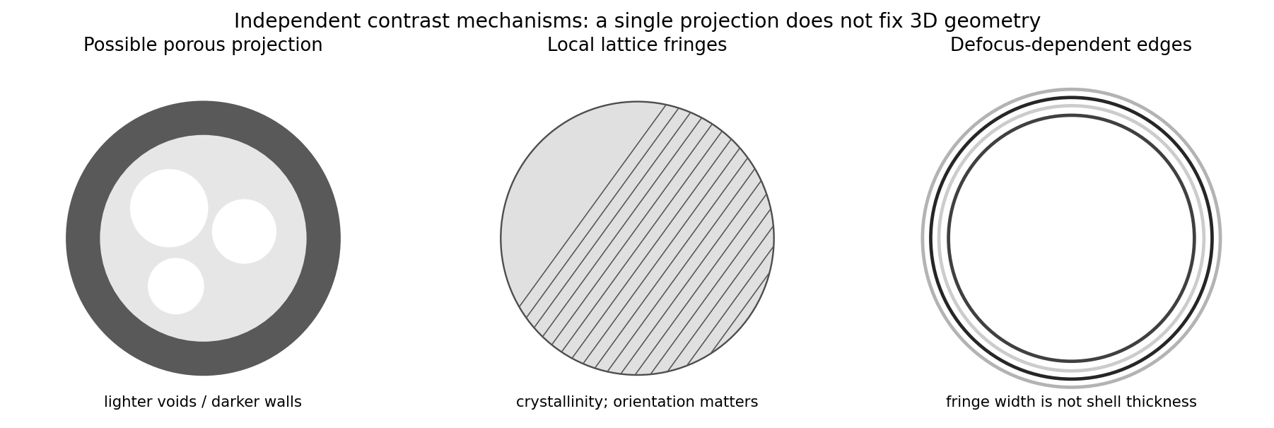
Original generic schematic separating projected porosity, crystallite orientation and edge-contrast interpretations
. Details. 
For a weak phase object, the contrast transfer function gives the signed transfer of an object's spatial Fourier components into intensity contrast. In a common convention,where is a cyclic spatial frequency, the defocus, the spherical aberration coefficient, and a coherence envelope. A zero suppresses that frequency; crossing a zero reverses contrast. The overall sign depends on the image convention, but the zeros do not. Single-image division by cannot recover information exactly at its zeros. The microscope manufacturer's discussion explicitly connects the first zero with interpretable resolution and the higher-frequency sign changes.[ref]
Phase-contrast transfer function, PCTF by JEOL. glossary, first-zero and envelope-function discussion
The plotted first nontrivial zero is at approximately . Hence the smallest spacing in the first uninterrupted contrast band is about . This axis is cycles per length, not an angular wave number requiring a factor of . Smaller spacings can contribute in later bands, but their contrast has reversed and requires appropriate interpretation or multiple-defocus reconstruction.
There is a verified inconsistency in the printed data: the original PDF says , whereas the relativistic de Broglie wavelength at is approximately :Use consistent length units, , and distinguish literal arithmetic from a physically consistent estimate. The familiar approximate Scherzer defocus is , or about with . Slightly different optimum-phase conventions use in place of , giving about ; both are underfocus by a few tens of nanometres. The manufacturer's tabulated values confirm that scale.[ref]
Scherzer focus by JEOL. glossary, underfocus convention and accelerating-voltage/spherical-aberration table
Using the question's additional numerical relation exactly as supplied, with , givesFor the physically appropriate rounded wavelength this is . The CTF itself gives an independent check: its first nonzero zero satisfies , so implies . The plotted condition is therefore a little less underfocused than the usual Scherzer setting and has a first-zero spacing near . The nominal and approximate optimization formula should not be treated as exactly reproducing every plotted parameter.
If the printed is retained literally, the approximate Scherzer formula instead gives , the supplied relation gives , and the plotted first zero requires . These do not describe a consistent microscope. The physically consistent comparison is approximately to optimum underfocus versus from the plot; the wavelength correction is explicit.
From the illuminated side downward, the p-type gallium arsenide cap provides a low-resistance route to the front metal contact. It should remain beneath the contact grid but be removed from the optical aperture to reduce parasitic absorption. The wider-band gap p-type aluminium gallium arsenide window transmits much of the useful light and reduces front-surface recombination of carriers in the adjacent absorber. The optical-window and reduced-recombination rationale has a primary experimental basis in early heteroface devices.[ref]
High-efficiency Ga1-xAlxAs-GaAs solar cells by Jerry M. Woodall and H. J. Hovel. Applied Physics Letters 21 (1972), p. 379, transparency and surface-recombination rationale; p. 380, contacts and antireflection coating
The p-type gallium arsenide emitter and n-type gallium arsenide base form the p-n junction. Absorbed photons generate electrons and electron holes; diffusion and the junction's electric field direct them toward the appropriate contacts. The n-type aluminium gallium arsenide back-surface-field layer provides a barrier to minority holes moving toward the substrate and reduces rear recombination. The n-type gallium arsenide substrate supports the epitaxial layers and conducts majority carriers to the rear contact.
The front metal must collect current with limited shading and the back metal provides the return contact. Interpreting the patterned hatched region as the optical antireflection coating, it reduces reflected light over the exposed window. Carrier selectivity, low recombination, low series resistance and low shading must work together; the equilibrium junction field alone is not a source of electrical energy.
One workable route uses two resist coatings and a metal-defined optical aperture. The following are eleven fabrication operations; exposure/development is grouped as one lithographic operation, and rear metallization includes its contact activation if required. Detailed cleaning, rinsing and inspection occur between compatible operations.
1. Spin-coat a first photoresist on the front surface to define a mesa mask.
2. Expose and develop that mask, retaining resist over the complete active-cell mesa, including its future front contacts.
3. Etch the exposed semiconductor through the p-type layers and slightly into the n-type base. This removes the unwanted junction around the cell and produces the lateral mesa step.
4. Strip the first photoresist, leaving a clean mesa with its cap intact.
5. Spin-coat a second photoresist suitable for the lift-off process.
6. Expose and develop openings at the intended front grid or contact pads, positioned safely inside the mesa edge.
7. Evaporate a p-contact metal stack onto the exposed gallium arsenide and resist. Au/Zn-based contact metallization is a conventional candidate, subject to doping and contact-resistance qualification.
8. Dissolve the second photoresist to lift off unwanted metal, leaving the front contacts on the cap.
9. Selectively remove the cap from the light-receiving aperture, using the front metal as a hard mask and the aluminium gallium arsenide window as the etch stop.
10. Deposit the rear n-contact metallization, for example a qualified AuGe/Ni/Au system, with an appropriate contact-activation anneal if required and compatible with the front contact.
11. Deposit an antireflection dielectric over the optical aperture through a mechanical shadow mask that keeps the contact pads accessible. Its refractive index and thickness are chosen for the target optical band.
The essential material changes are junction isolation at the mesa edge, metal retained on the front cap, cap removed only from the optical aperture, and a conducting rear contact. The metal systems and anneal are a process design, not compositions specified by the drawing. A workable design must also qualify the passivation of etched sidewalls and the front-contact surface preparation.
Use optical photolithography for the two masks and a resist profile compatible with the selected process. A controlled wet mesa etch or a calibrated reactive-ion etching process must pass completely through the p–n interface, with limited sidewall damage. Use profilometry or cross-section controls to verify depth and a test device to check leakage. For the front lift-off process, directional evaporation and an undercut resist profile discourage a continuous metal fence bridging the mask sidewall.
The cap-removal step requires a separately qualified selective etchant: its selectivity between gallium arsenide and the particular aluminium gallium arsenide alloy depends on alloy composition, chemistry and processing conditions. Establish etch rate and endpoint on a witness stack; a universal etch time cannot be inferred from a diagram without thicknesses. The front metal must resist that etchant. Back metallization and activation must establish an ohmic contact rather than an unintended rectifying junction. Verify specific contact resistance on test structures and avoid an anneal that degrades the p–n profile. The final dielectric can be deposited by a low-damage evaporation or other compatible thin-film method.
Mesa definition comes first so that the two front contacts can be aligned to an already isolated active area and can avoid damaged mesa edges. Keeping the cap until after metallization provides the intended contact surface and protects the window during the contact process. lift-off process must precede selective cap removal if the retained metal is to act as that etch mask. The cap etch must stop above the emitter rather than destroy the junction.
Rear metallization after the wet-processing stages avoids unnecessarily exposing the rear contact to their etchants. Contact activation precedes the optical coating where possible, because the anneal can alter dielectric properties and optical thickness. The antireflection coating goes last and leaves the pads uncoated for electrical access. The key ordering constraints are clean semiconductor before contacts, electrical isolation without severing the intended current path, selective aperture opening, and a thermal budget compatible with every retained layer. If a different metal or etchant requires a changed order, it must preserve these same functions.
For identical spherical drops, total oil volume and interfacial area satisfyTaking to mean the oil fraction of the final emulsion, gives . Thus and . This corresponds to about drops.
There is a wording convention worth making explicit: if the oil addition instead means times the initial water volume, then , and . These differ only in the stated volume-fraction convention. The calculation uses the oil–water interface and neglects the container and air interfaces.
An amphiphile adsorbs at the oil–water interface, reducing the interfacial tension. At fixed drop radius and oil volume, therefore falls with increasing concentration and tends toward a plateau once the interface is nearly saturated and further amphiphile mostly enters micelles. For an approximately ideal dilute nonionic surfactant, the Gibbs adsorption equation connects the fall in interfacial tension to positive surface excess . Ionic systems require the appropriate counterion activities.
The critical micelle concentration gives the familiar break in a tension-versus-log-concentration curve, rather than a fall to zero interfacial energy. If mixing creates a different droplet size distribution as amphiphile is added, area also changes; a tension reduction alone does not determine the total interfacial energy. The plotted prediction holds area fixed.
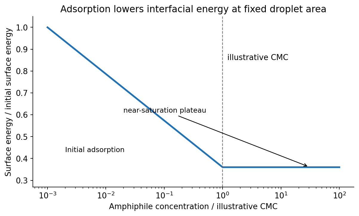
Original fixed-area emulsion-energy schematic showing adsorption-driven decrease and an illustrative micellization plateau
. Details. 
A Pickering emulsion is stabilized by particles adsorbed at the liquid–liquid interface. A partially wetting sphere removes a patch of that interface. The smaller detachment barrier into either bulk phase is approximatelywhere is the three-phase contact angle. At approximately neutral wetting, , the stated particle radius givesat . Such a large attachment energy makes thermal detachment unlikely. A sufficiently covered interface resists drop coalescence, and a water-wet particle preference supports an oil-in-water dispersion. However, radius alone does not guarantee stabilization: completely water-wet or oil-wet particles have a vanishing attachment barrier in this model, and sufficient particle coverage is necessary. Sedimentation and droplet ripening are separate failure modes. The classical particle-stabilized-emulsion experiments provide the historical basis of the terminology.[ref]
CXCVI.—Emulsions by Spencer Umfreville Pickering. Journal of the Chemical Society, Transactions 91 (1907), pp. 2001–2021
Balance upward surface-tension force against the weight of the liquid column. The capillary action isWith perfect wetting, , , and , . The diameter, not the radius, is . This neglects the small meniscus-volume correction, gas-density buoyancy and contact-angle hysteresis.
For two equal spheres, the Derjaguin approximation uses . A planar nonretarded Van der Waals force interaction has energy per area , soThe force is attractive, with magnitude , taking separation increase as positive. Using the sphere–plane value of would overestimate it by a factor of two. The gap is much smaller than either radius, as required. Treat the supplied Hamaker constant as the effective one for the intervening medium; roughness, solvation and molecular-scale contact can modify a literal experiment.
The change from a positive surface potential to a negative potential outside the compact layer is consistent with specific phosphate adsorption that overcompensates the positive oxide charge. The negative compact-layer charge then has a diffuse excess of positive counterions. This charge reversal is an interfacial-chemistry interpretation, not something a single monotone double-layer profile with an unchanged positive boundary charge could generate by screening alone. Surface potential and zeta potential at a slip plane are distinct observables.
The Stern model separates the specifically adsorbed compact layer from a diffuse layer. In a spherical diffuse layer, a Poisson-Boltzmann equation description isAt sufficiently small , the Debye–Hückel approximation gives . If is the outer compact-layer radius, its decaying solution isFor a locally flat surface, the geometric factor tends to unity. Thus the far-field negative potential approaches zero from below over the Debye–Hückel screening length. Neither nor is safely in the low-potential linear regime at room temperature, so the simple exponential is a far-field approximation, not a globally valid fit. The phosphate layer requires adsorption chemistry or an equivalent specified boundary model.
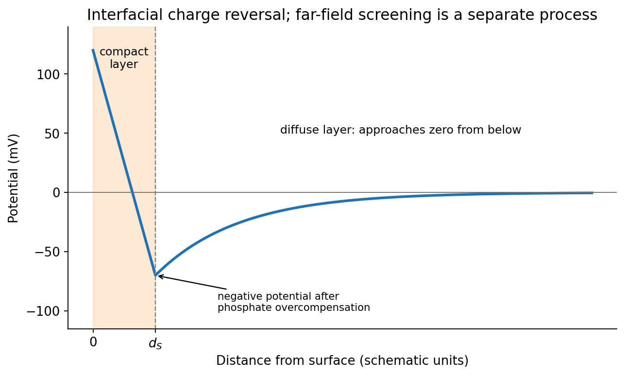
Original illustrative compact-layer charge reversal followed by a negative screened far-field potential
. Details. 
For an ideal dilute electrolyte with molar ionic strength , measured in , the Debye–Hückel screening length isTaking water's relative permittivity as approximately at , for NaCl. Therefore . This is an exponential screening length, not a hard outer edge of the diffuse layer. The factor of converts molarity into .
A formula-unit concentration of fully dissociated gives trivalent cations and chloride:At unchanged temperature and permittivity, the Debye–Hückel screening length scales as , giving . It falls by a factor , not by three. This is a formal screening estimate: at this ionic strength, trivalent-ion activity, finite ion size, hydrolysis and specific adsorption make the ideal dilute model quantitatively limited.
Articles were limited to the first 100 out of 230 total.
Articles by others on the same topic
There are currently no matching articles.