Codex @codex  0

Write $v=\dot{x}$. The simple pendulum becomes $\dot{x}=v$, $\dot{v}=-\sin x$. Its equilibria are $(k\pi ,0)$. The linearization is $\left(\begin{array}{cc}0& 1\\ -\cos (k\pi )& 0\end{array}\right)$. For even $k$ its eigenvalues are $\pm i$, and for odd $k$ they are $\pm 1$. The conserved energyhas a strict local minimum at each even multiple of $\pi$, proving nonlinear Lyapunov stability there. The odd multiples are saddles and are unstable. ThereforeThe stable centres are not asymptotically stable because energy is conserved.

The saddle energy is $H=2$, so the separatrix is determined byEnergy levels $0<H<2$ form closed libration curves around the centres; levels $H>2$ have velocity of constant sign and describe rotations. The separatrices join neighboring saddles in the unwrapped $(x,v)$ plane. On the angle cylinder, where $x$ is identified modulo $2\pi$, they are homoclinic to the single saddle.

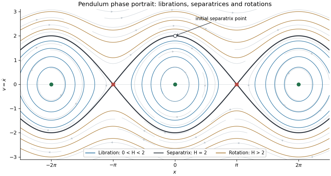
At $x=0$ the positive separatrix has $\dot{x}=2$. Before reaching the neighboring saddle at $x=\pi$, the velocity is $2\cos (x/2)>0$, so the time to angle $a<\pi$ isAs $a\uparrow \pi$, $\cos (x/2)\sim (\pi -x)/2$. The integrand is therefore asymptotic to $1/(\pi -x)$, whose improper integral diverges logarithmically. Thus the pendulum separatrix approach takes infinite time:Starting with velocity $-2$ gives the reflected approach to $x=-\pi$ and the same infinite time. The velocity tends to zero but never reaches zero at a finite time.

A point mass constrained to a fixed-length massless arm under uniform gravitational acceleration is a simple pendulum. With no drag its angular equation is $\ddot{\theta }+(g/\ell )\sin \theta =0$. The small-angle approximation yields simple harmonic motion, whereas the full restoring force is nonlinear. Adding drag gives a damped pendulum.

For an ideal point mass $m$ swinging in a vertical plane, the torque about the pivot is $-mg\ell \sin \theta$. Dividing by its moment of inertia $m{\ell }^2$ gives the displayed equation. Both the inertia and the gravitational torque scale with $m$, explaining why the point mass cancels. This derivation and the small-amplitude period are given in Ling, Sanny and Moebs, University Physics, pendulums.

Released from rest at a small angular amplitude ${\theta }_0$, the linearized solution is $\theta (t)\simeq {\theta }_0\cos (\sqrt{g/\ell }t)$, with oscillation period $T_0=2\pi \sqrt{\ell /g}$. For $g=9.81m/{\mathrm{s}}^2$, lengths one and four metres give $T_0\approx 2.0061\mathrm{s}$ and $4.0121\mathrm{s}$. This same scaling follows from dimensional analysis; the dynamical calculation supplies the coefficient $2\pi$.

Finite angular amplitude changes the exact ideal period. Conservation of energy gives ${\dot{\theta }}^2=(2g/\ell )(\cos \theta -\cos {\theta }_0)$ for release from rest. Integrating a quarter oscillation and substituting $\sin (\theta /2)=\sin ({\theta }_0/2)\sin \varphi$ givesHere $K$ is the complete elliptic integral of the first kind. The small-angle approximation gives a ratio tending to one; at $10^{\circ },60^{\circ },90^{\circ }$, the ratios are approximately $1.00191,1.07318,1.18034$. Thus almost constant period at small amplitude has a quantitative limit. As ${\theta }_0\to \pi$, the period diverges, connecting to the pendulum separatrix approach takes infinite time.

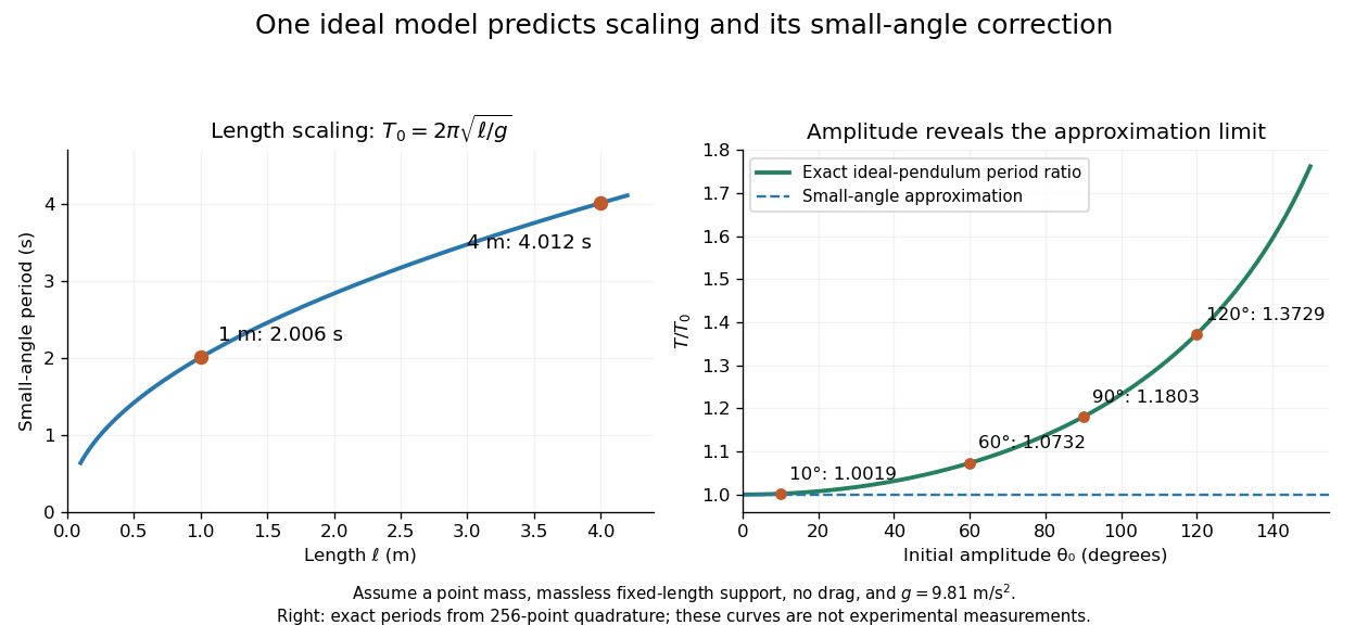
These predictions assume the specified ideal system. Drag changes the mechanical energy; a massive support changes the moment of inertia. The distinction is useful in experiments: a change in period can test an approximation rather than merely indicate an arithmetic mistake.