A point mass constrained to a fixed-length massless arm under uniform gravitational acceleration is a simple pendulum. With no drag its angular equation is . The small-angle approximation yields simple harmonic motion, whereas the full restoring force is nonlinear. Adding drag gives a damped pendulum.
For an ideal point mass swinging in a vertical plane, the torque about the pivot is . Dividing by its moment of inertia gives the displayed equation. Both the inertia and the gravitational torque scale with , explaining why the point mass cancels. This derivation and the small-amplitude period are given in Ling, Sanny and Moebs, University Physics, pendulums.
Released from rest at a small angular amplitude , the linearized solution is , with oscillation period . For , lengths one and four metres give and . This same scaling follows from dimensional analysis; the dynamical calculation supplies the coefficient .
Finite angular amplitude changes the exact ideal period. Conservation of energy gives for release from rest. Integrating a quarter oscillation and substituting givesHere is the complete elliptic integral of the first kind. The small-angle approximation gives a ratio tending to one; at , the ratios are approximately . Thus almost constant period at small amplitude has a quantitative limit. As , the period diverges, connecting to the pendulum separatrix approach takes infinite time.
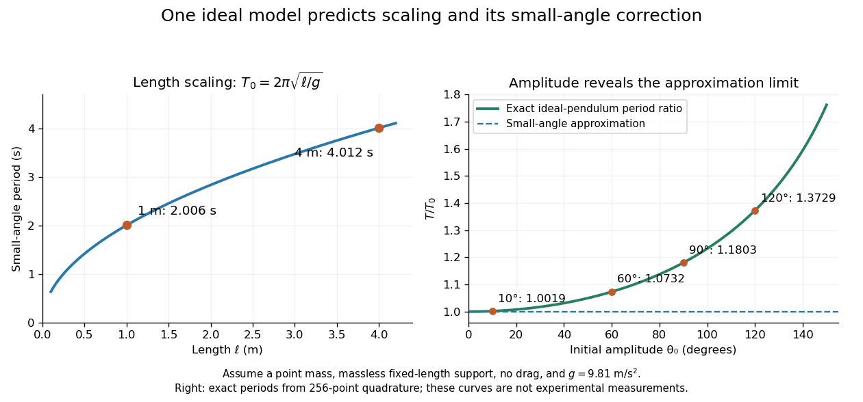
These predictions assume the specified ideal system. Drag changes the mechanical energy; a massive support changes the moment of inertia. The distinction is useful in experiments: a change in period can test an approximation rather than merely indicate an arithmetic mistake.
A point mass constrained to a fixed distance from a pivot and free to move in three dimensions under uniform gravitational acceleration. With the vertical axis downward and polar angle measured from it, the Lagrangian is the expression in the title. The azimuth is a cyclic coordinate, so is conserved angular momentum about the vertical axis. A rigid massless rod enforces the constraint without the loss-of-tension limitation of a string.
For a spherical pendulum with nonzero conserved vertical angular momentum , eliminate the azimuthal angular velocity using . The polar effective potential is . A conical pendulum at is a minimum satisfying . Linearization at fixed yields polar angular frequency , where is the conical revolution frequency squared. Holding fixed during the perturbation would describe a different, externally driven constraint. The polar perturbation is a nutation; the exactly planar limit requires separate treatment.
Two identical planar simple pendulums of length and bob mass , with pivots separated horizontally by , are coupled by a straight spring of natural length and spring constant . In the ideal model without contact restrictions, their configuration space is the torus . Measure both angles from the downward vertical towards the same horizontal direction. Their bob separation isThe exact Lagrangian is the expression in the title. To derive it, use bob positions and . Kinetic energy from Cartesian position vectors gives . Gravitational potential energy is and spring potential energy is ; subtracting these from proves the formula. Near the downward equilibrium, for fixed , giving the familiar normal modes of two spring-coupled equal pendulums.
For support displacement and angle measured from the downward vertical, the mass position is . Its Euler-Lagrange equation is . In the support frame the effective acceleration is ; taking its torque about the hinge gives . The prescribed support can do work, so pendulum energy need not be conserved.
For small angles about the downward vertical and prescribed pivot position , a simple pendulum obeys the displayed forced-oscillator equation. Off resonance, its harmonic particular solution is , with . At exact resonance, a pendulum initially vertical with zero angular velocity has in the undamped linear model. The growing envelope eventually violates the small-angle assumption; damping and nonlinear frequency shifts matter in a real pendulum.
For a small, rapid horizontal displacement , the leading fast angular excursion is . Correlating that excursion with the driving torque gives the averaged force . Its effective potential is . The downward state loses linear stability above and two tilted minima appear. Small and slow dynamics compared with are required; horizontal and vertical support vibration produce different effective potentials.
Inside a spherical body of uniform density, the shell theorem gives gravitational acceleration . A simple pendulum at depth therefore has period . If its clock is calibrated at the surface, its indicated elapsed time is and it loses . This is a mechanical clock-rate change caused by weaker local gravity, not gravitational time dilation. The uniform-density assumption is essential; Earth's actual density profile gives a different interior field.
A conical pendulum is a pendulum whose bob executes uniform horizontal circular motion beneath a fixed pivot, with its string at a constant angle to the downward vertical. The string sweeps a right circular conical surface; the bob follows its circular rim, without any physical cone supporting it. The ideal model has a point mass , a taut, massless, inextensible string of length , uniform gravitational acceleration of magnitude , and negligible drag force and pivot friction. A nonzero circular motion requires . This geometry and the corresponding forces are described in Richard Fitzpatrick, The conical pendulum, equations 262–267.
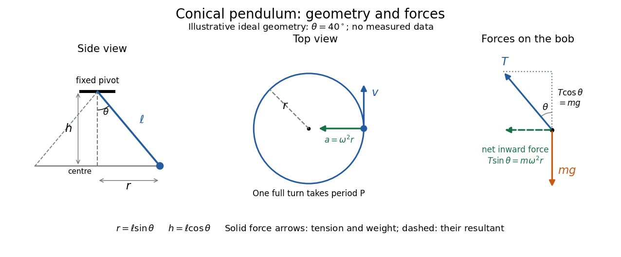


The right triangle formed by the pivot, the orbit centre, and the bob gives and . Here is the orbit radius and is the vertical drop from the pivot to the bob's horizontal plane, not the bob's height above a table. Write for tension, for the oscillation period of one revolution, and for the angular speed; then the bob's speed is . A side view compresses the horizontal circle to a line segment; the top view reveals the circle and its tangent velocity.
The two actual forces on the bob are tension toward the pivot and gravitational weight vertically downward. The vertical acceleration is zero, while the horizontal centripetal acceleration is . Thus Newton's second law givesThe inward net force is the horizontal component of tension, rather than an extra interaction to add to these two forces. Constant speed still requires acceleration because the velocity changes direction. [ref]
https://openstax.org/books/university-physics-volume-1/pages/6-3-centripetal-force. Ling, Sanny and Moebs, University Physics 1, §6.3: centripetal acceleration and net force
Dividing the two component equations and using gives the useful collection of predictionsIf is the azimuthal angle, then ; either direction of rotation satisfies . The mass cancels from the angular speed and oscillation period, but not from the tension. The motion is a relative equilibrium: in a rotating frame following the bob at angular speed , its position is fixed. This is a concrete way to see how rotational symmetry can turn an apparently moving solution into a stationary one.
A conducting conical pendulum connected to a grounded pivot develops a motional electric potential difference between the rotation axis and a bob at radius . If the bob dominates the capacitance, its electric charge is . An additional uniform vertical electric field changes both the force on that charge and, while the grounding connection remains, the background electric potential entering the charging relation. These effects must be treated consistently when calculating a first-order mechanical response.
The motivating observation is a bob going around at almost constant height while its string traces a cone. The University of Iowa's demonstration places a camera above a short pendulum to reveal this motion. [ref]
https://instructional-resources.physics.uiowa.edu/1d5025-conical-pendulum. University of Iowa, demonstration 1D50.25: short pendulum and overhead camera
The following proposed measurement procedure develops that observation into a test of the conical pendulum model; it is not a report of collected data.Suspend a compact bob from a rigid, fixed support using a light string, and measure from the pivot to the bob's centre. Put a stationary marker beside the orbit as a timing reference. Displace the bob sideways and give it a horizontal push tangent to the intended circle, then let go. For a chosen starting angle , the predicted initial speed is . Adjust the launch between trials until a short observation interval has nearly constant orbit radius and height. Keep the pivot fixed while recording: circling the support by hand changes the problem, and a maintained drive would introduce another force.
Record from above with the camera looking approximately along the vertical axis. Check that the bob's centre follows a circle and that successive returns to the marker take nearly equal times. A separate side recording checks whether the bob's height stays constant. A markedly elliptical orbit or visibly rising and falling bob is not the uniform circular motion assumed by the conical pendulum equations. Measure the orbit diameter with a scale at the orbit's height; in a level side view, use the two extreme horizontal positions, not one arbitrary frame. Halve the diameter to obtain , or measure the vertical drop directly in a calibrated side view. An oblique camera view and a scale at a different depth distort apparent lengths, so arrange the geometry before interpreting the images.
Time complete returns to the same marker in the same direction and estimate . Counting ten revolutions, when the orbit stays sufficiently steady, spreads an endpoint timing error over ten periods. Repeat the timing and compare the first and last few revolutions to detect drift; using a longer interval helps only if the motion remains close to uniform. From independently measured geometry, compute or , and check if both were measured. Then compare the measured oscillation period with . MIT's 8.01X experimental assignment explicitly asks students to compare the conical pendulum's period, length, and orbit radius with theory. [ref]
https://ocw.mit.edu/courses/8-01x-physics-i-classical-mechanics-with-an-experimental-focus-fall-2002/a056f6a3e071767d4f7620bca6a59d0c_expt_vs_problem.pdf. MIT 8.01X, Fall 2002, Vibrating Systems experimental problem, question 8
Repeat at several launch radii with the same . Larger means smaller , so the ideal oscillation period decreases. A plot of measured against independently measured should follow a straight line through the origin with slope ; conversely, estimates gravitational acceleration. Do not infer from the timing equation and then use that same equation as a test. Compare discrepancies with the spread of repeated timings and the resolution of the length measurements. String stretch, a moving pivot, and appreciable bob size challenge the stated geometry; drag force and pivot friction challenge the assumption of undriven uniform motion. Observe a short interval and record any shrinking or drifting orbit rather than silently treating it as an exact conical pendulum.
For an illustrative calculation, assume , , , and . The model gives , , , , and . Its vertical tension component is , equal to the gravitational weight; its inward component is approximately . These are predictions from chosen parameters, not measured data or measurements of local . The next figure uses the same stipulated and , including illustrative angles , , and .
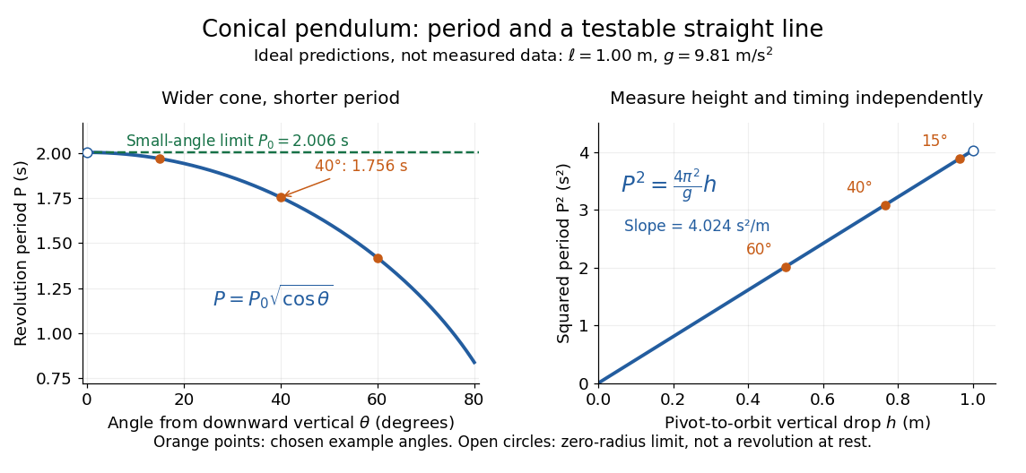
Ideal conical pendulum period decreases with cone angle and its square is proportional to the vertical drop
. Details. 
For fixed and , the exact conical pendulum oscillation period satisfies . In the small-angle approximation, with in radians,Thus the limiting revolution period equals the small-amplitude oscillation period of a planar simple pendulum. This equality has a geometric explanation: to first order, and are perpendicular simple harmonic motions of equal amplitude, a quarter period apart, with . At finite angle, however, the conical pendulum's oscillation period decreases with , whereas a planar simple pendulum's oscillation period increases with its angular amplitude.
The endpoint itself is a stationary bob with and no observable revolution; is a limit of nonzero circular motions, not a measured revolution period at rest. For fixed , nonzero conical pendulum motion also requires , because . At the other endpoint, gives , , and unbounded tension and speed. These mathematical limits explain why the ideal string cannot sustain a horizontal orbit at finite tension; a real experiment ceases to satisfy the ideal assumptions before that limit.
A damped pendulum is a simple pendulum whose mechanical energy is removed by a resisting torque. Here the model is undriven, with a fixed pivot, a point mass at distance , uniform gravitational acceleration , and resisting torque with constant . The angle is measured from the downward vertical in radians. An ideal viscous rotary dashpot realizes this torque law; tangential linear drag on the bob gives the same equation with . The moment of inertia is , soHere is physical time, is the undamped small-amplitude angular frequency, and has units of inverse time. In the normalized equation , dots mean differentiation with respect to , not . The parameter is dimensionless. This separates the chosen damping law from the small-angle approximation: retaining allows finite angles even when the resisting torque is linear in angular velocity.
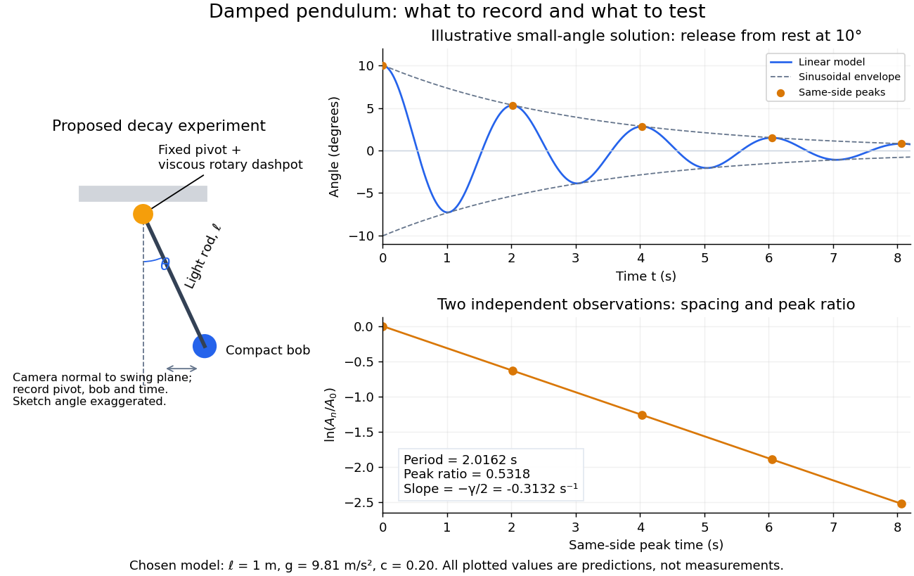
Proposed viscous-damper experiment and illustrative small-angle decay: angle versus time and successive peak ratios, not measured data
. Details. 
To motivate the model, release a pendulum without a push and record how its swing shrinks. A published example by Gintautas and Hubler uses a rotary sensor built from a computer mouse to measure the frequency and damping coefficient of a physical pendulum. [ref]
https://arxiv.org/abs/0901.4319. Gintautas and Hubler, A simple, low-cost, data-logging pendulum built from a computer mouse, 2009
The following is a proposed experiment with a chosen viscous rotary dashpot; the plotted observations are predictions, not a reproduction of their measurements.Mount a compact bob on a light rigid rod with a fixed pivot, couple the pivot to an adjustable viscous rotary dashpot, and measure from the pivot to the bob's centre. First record decay with the dashpot disconnected, then repeat with it connected at several settings; this establishes how much decay is already due to other losses. Keep the bob, rod, camera, and release angle unchanged between these trials. The simple model requires rod and damper-rotor moments of inertia to be negligible compared with . Otherwise measure the total moment of inertia and the distance to the assembly's centre of mass: the physical pendulum equation becomes , where is the total moving mass. A damper that also exerts an elastic restoring torque would require another term.
Place a camera perpendicular to the swing plane, include the pivot and bob centre in every frame, and determine their coordinates relative to the resting vertical. For horizontal and downward separations , use ; record the frame timestamps rather than assuming a frame rate. Release from rest at about , record through several complete swings, and repeat the release. For every same-side turning point, tabulate its time and angular amplitude . Measure the oscillation period from differences ; comparing several periods exposes drift. Interpolating around each observed extremum reduces frame discretization error. Check that late peaks still exceed the angular resolution; taking the natural logarithm of tiny, uncertain peaks amplifies their relative errors.
In the small-angle approximation, the damped pendulum becomes a damped harmonic oscillator. For and release from rest at , its exact linear-model solution isThe decaying sinusoidal envelope has coefficient ; because release is from rest, its successive same-side extrema occur at and have . Thus the envelope and the sequence of actual peak heights are different descriptions of the same trace. The linear damping regimes and this solution are derived in Richard Fitzpatrick, Damped Oscillatory Motion, equations 82–93.
The experiment tests two predictions independently: nearly equal same-side peak spacing and a straight line when plotting against . Its predicted slope is , givingUse several peaks and repeated trials rather than a single ratio, and compare the frequency identity with independently measured and . For the illustrative choices , , , and , the linear model gives , , and . The first two positive peaks after release are therefore approximately and . The undamped small-amplitude oscillation period is about : substantial loss per swing need not imply a large change in period.
Repeat at a larger release angle to distinguish two limitations. The relative error in replacing by is about for small angles: about at , but about at when compared with . Finite-amplitude swing spacing can therefore change as the swing shrinks even if is constant. Separately, friction at the pivot or quadratic drag can invalidate the assumed linear resisting torque; exponential peak decay should be checked, not imposed on all recorded motion. Peters discusses why real pendulum damping can require nonlinear terms. [ref]
https://arxiv.org/abs/physics/0306081. Randall D. Peters, Nonlinear Damping of the 'Linear' Pendulum, 2003
Repeatability, residual pivot motion, changes in damper temperature, and finite camera resolution are useful checks on this proposed measurement.The normalized equilibrium points are . Even multiples of are attracting: their linearization has eigenvalues , giving a stable focus for , repeated negative eigenvalues at , and a stable node for . These are the underdamped, critically damped, and overdamped small-displacement regimes. Odd multiples of have eigenvalues of opposite signs and are saddle equilibria. The energy dissipation of a damped pendulum explains why trajectories in the phase portrait spiral inward near a stable focus instead of closing into the recurring orbit of an undamped simple pendulum.
For the normalized damped pendulum, the sum of kinetic energy and gravitational potential energy, divided by , isThe chain rule and the full nonlinear equation give this identity exactly, without a small-angle approximation. Here as in damped pendulum. In physical units the mechanical energy and the power of the resisting torque areThe pendulum's lost mechanical energy is transferred to the damper and surroundings; it does not violate conservation of energy. In an ideal viscous dashpot this loss is frictional heating. The exact cumulative balance is particularly useful for checking a numerical solution:
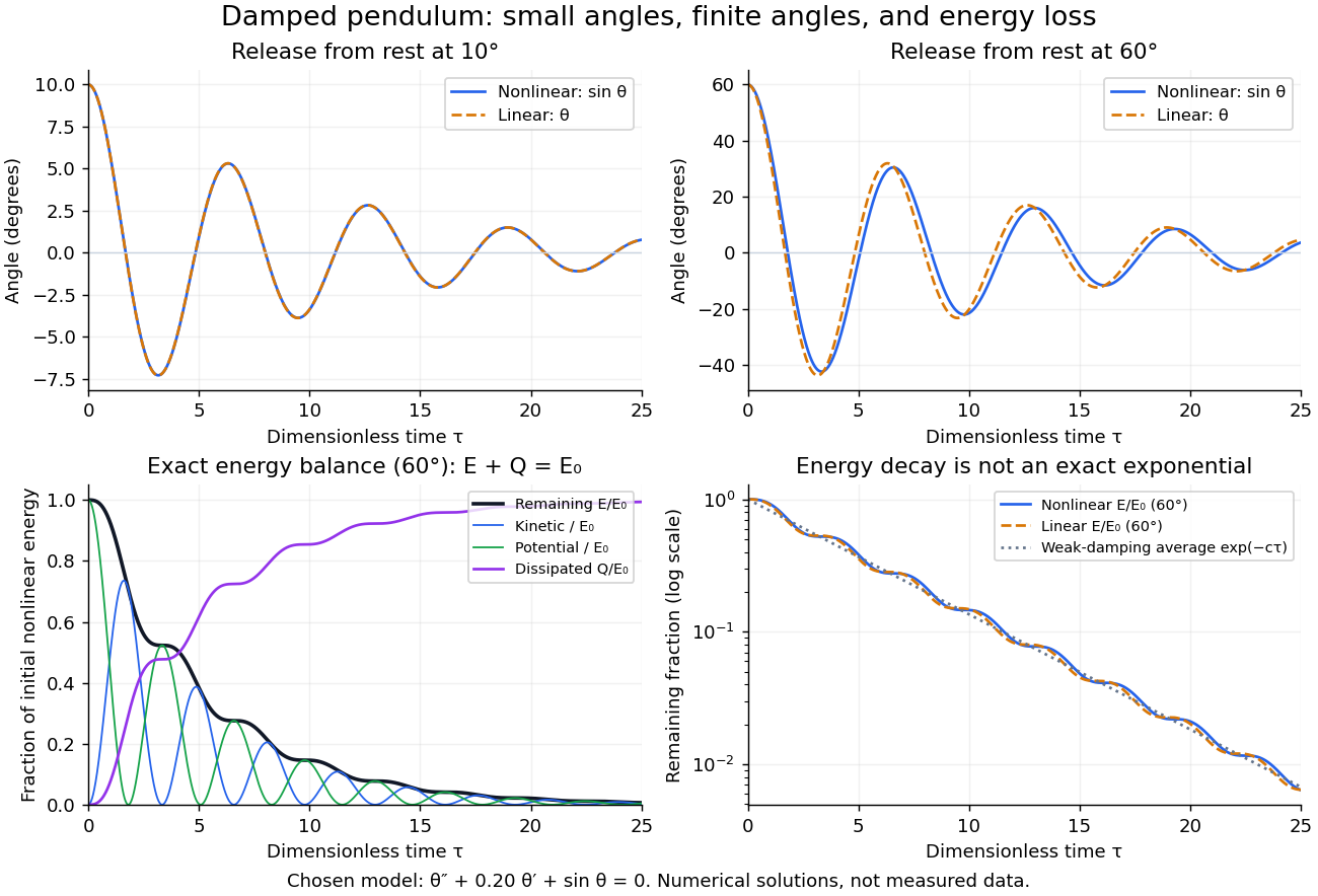
Illustrative nonlinear and linear damped pendulum solutions at 10 and 60 degrees, with exact mechanical energy transfer and loss; no measured data
. Details. 
The figure uses and release from rest. Over , the largest angular discrepancy between the nonlinear solution and the damped harmonic oscillator solution is approximately () for a release, but () for a release. Their nonlinear initial energies are and , respectively. At the remaining fractions are approximately and . These are illustrative calculations from specified initial conditions, not observations. The generator uses a Runge-Kutta method and integrates alongside the motion; halving its step and independently integrating checks the result.
For and , the first three nonlinear same-side swing intervals after a release are approximately , , and . They approach the linear-model oscillation period as the amplitude shrinks. After a release the corresponding intervals are already about , , and . This makes the experiment's period drift a quantitative test of the small-angle approximation, rather than an automatic reason to change the damping coefficient.
At a turning point, and even though the swing is losing mechanical energy over the cycle. Its potential energy there is , so measured turning angles give successive energies without estimating angular velocity. In the proposed decay experiment, multiply these values by to obtain energies in joules, then subtract adjacent same-side energies to estimate the loss over each full swing. Only for small amplitudes is . In the linear underdamped model, same-side peak energies consequently satisfy , the square of the angular amplitude ratio. For the illustrative parameters above this energy ratio is approximately . Between turning points, kinetic energy and potential energy continue to exchange while their sum decreases; the energy slope vanishes briefly at each extremum and is negative whenever the bob moves.
It is therefore inaccurate to replace the exact identity by . Even for the linear model, has . For weak damping and small angles, cycle averaging gives , so the averaged energy approximately follows while angular amplitude follows . This exponential decay is an approximation to the energy trace; the same-side peak ratio is exact within the linear model. The figure distinguishes the actual energy curves from this averaging approximation.
The energy identity also gives a global conclusion without solving the nonlinear equation. If were constant on a positive-length interval, then would vanish throughout it; the equation would force , making the entire trajectory an equilibrium. Every nonstationary trajectory therefore loses mechanical energy over every positive-length interval, even though its instantaneous derivative can vanish at a turning point. A nonconstant periodic motion would have to return to its initial mechanical energy, so it is impossible for this undriven damped pendulum. Oscillations near a stable focus are successive, shrinking swings, not a repeating cycle. Moreover, if , the angle cannot reach an upright equilibrium, whose potential energy is ; such motion stays within its original potential well. This is the usefulness of the energy description: one scalar balance controls both the observed decay and which nonlinear motions remain accessible.
A Foucault pendulum is a long simple pendulum whose suspension allows the bob to swing in both independent horizontal directions. Its slowly changing swing direction relative to the building reveals Earth's rotation. A hinge restricting the bob to one vertical plane would prevent this measurement: the support would impose the very direction we want the pendulum to select freely. Léon Foucault demonstrated the effect in 1851.[ref]
The bob's back-and-forth oscillation and the swing direction's precession are different motions. The bob traverses its arc in seconds, while successive arcs change direction over hours. In a conical pendulum the bob itself circulates around the vertical; a nearly planar Foucault pendulum instead reverses along an almost straight horizontal trace, whose orientation changes slowly. The measured quantity is that orientation against a fixed floor or wall reference, rather than the bob's instantaneous azimuth.
The University of New South Wales documents an undriven, visitor-started Foucault pendulum. A fixed vertical wire and wall line define its initial north–south swing plane. The documented comparison one hour later shows reduced amplitude and about nine degrees of anticlockwise precession. The apparatus swings for several hours without an electromagnetic drive.[ref]
The Foucault pendulum by Joe Wolfe. The Foucault pendulum, opening observation sequence and Our Foucault Pendulum: wire/wall reference, one-hour comparison, no electromagnetic drive
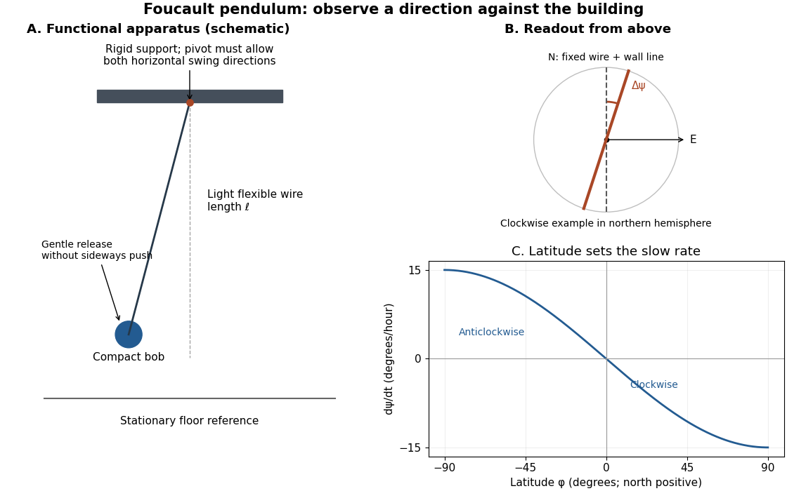
Functional Foucault pendulum apparatus, fixed sighting reference, and predicted latitude dependence; schematic with no historical dimensions
. Details. 
To turn that demonstration into a quantitative experiment, the following is a proposed measurement protocol. Establish a rigid support with no preferred horizontal swing direction, measure the wire length to the bob's centre, and mark two perpendicular horizontal axes fixed to the building. Start with a small displacement along the sighting plane, then release with as little transverse velocity as possible. Record the actual launch method; burning a fine restraining thread is one possible proposed release, not a claim about the documented UNSW launch. Keep people clear of the bob and avoid touching the suspension during the observation.
Record the horizontal position from above with a stationary, calibrated camera, or sight the bob against the wire and wall line at recorded times. Fit the long axis of each short group of swings to estimate its orientation ; use the extrema on both sides rather than following the bob's rapidly reversing velocity. A swing line has orientation modulo , so unwrap successive small direction changes continuously. Rotate no camera or reference between measurements. Record the fast oscillation period separately, and compare the slope of with the Latitude law of Foucault precession. Repeat launches along different directions and monitor ellipses, pivot motion, and air currents before attributing the slow change to Earth's rotation.
Use local east, north, and up unit vectors, with eastward, northward, and positive orientation anticlockwise as viewed from above. Let be signed geographical latitude, positive north, and the magnitude of Earth's angular velocity. In the spherical-Earth approximation,Here is the local effective gravity in a rotating frame, including the steady terrestrial centrifugal acceleration. For small horizontal displacements compared with , the horizontal restoring acceleration from tension is . Vertical displacement is second order in the swing amplitude, so vertical velocity can be omitted at this order. The horizontal Coriolis acceleration in local Earth coordinates then gives the coupled linear differential equationsThese equations neglect damping, finite-amplitude corrections, support anisotropy, and spatial changes of the centrifugal force of order ; they retain the leading terrestrial Coriolis force. A related derivation uses south/east axes instead.[ref]
Foucault's pendulum - the physics (and maths) explained by Joe Wolfe. Foucault's pendulum - the physics (and maths) explained, equations (9.1*)–(11): horizontal small-oscillation equations
Introduce the complex number . Multiplying the second equation by and adding givesSet . Direct differentiation cancels the first derivative of and yieldsThe in comes from solving these reduced equations exactly; it is not a complete prediction of terrestrial corrections of order . Thus the horizontal trajectory is an ellipse in coordinates rotating at angular velocity relative to the building. When , each rapid swing samples an almost fixed long axis; its slow precession isThe sidereal day is a rotation relative to distant directions. denotes a full turn of a continuously followed orientation; an unlabelled swing line repeats after . At the equator there is no finite precession period in this model. The Coriolis parameter is , so the plane's rate is , not .
The limiting cases check the sign and scale. At the north pole : the swing direction turns clockwise once per sidereal day. At the equator : both horizontal equations reduce to independent simple harmonic motions and a line launch stays on its original line. At the south pole : the direction turns anticlockwise once per sidereal day. Vanishing horizontal precession at the equator does not mean that every component of Coriolis acceleration vanishes there.
For a stipulated , the sidereal day is approximately . At north the predicted rate is and ; at south the rate changes sign. At the illustrative geographical latitude south, the prediction is . These calculations are model predictions, not new observations of the UNSW apparatus.
A swing plane fixed among the stars is generally only a polar picture. A north–south swing at the equator turns with Earth in an inertial frame, while having no precession against the building.[ref]
The Foucault pendulum by Joe Wolfe. The Foucault pendulum, The 'plane' of the pendulum's swing is not fixed in space: equatorial counterexample
For release from rest relative to the building, take , . The exact solution of the stated coupled linear differential equations isIndeed and , so . In the slowly rotating coordinates, the ellipse has semiaxes and . A bob released from rest therefore does not describe a perfectly straight line even in this ideal linear model. Replacing the bracket by gives the familiar leading approximation but introduces a spurious initial transverse velocity . The exact expression keeps the initial condition and separates that tiny orbit width from the slow rotation of its long axis.
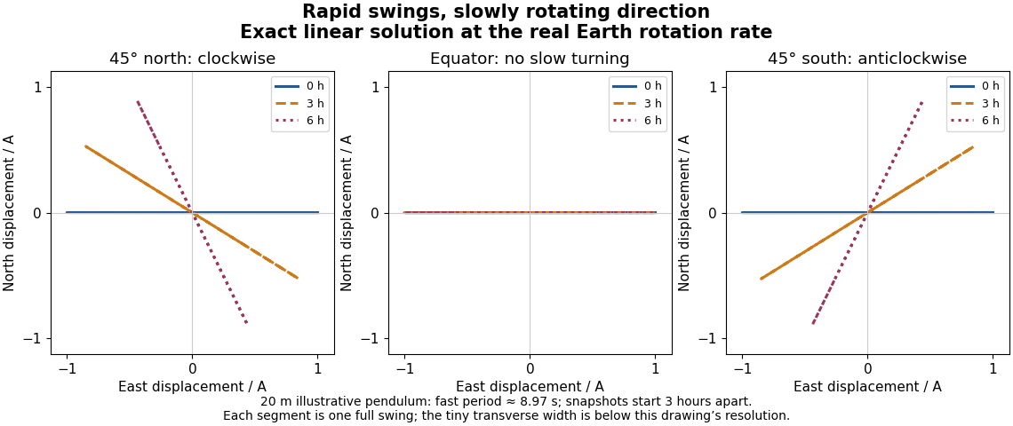
Exact trajectories of the linear Foucault pendulum equations at the actual Earth rotation rate, showing one swing near zero, three, and six hours at northern, equatorial, and southern latitudes
. Details. 
For the illustrative and , the fast period is approximately . At north, : the transverse semiaxis is too small to distinguish at the figure's scale. Nevertheless the long-axis orientation changes by about in six hours. Changing the sign of geographical latitude conjugates the entire solution, reflecting the trajectory across the eastward axis; setting gives exactly. These are stronger checks than merely drawing a rotating line.
The coupled equations give an additional independent constraint. Multiplying them by and and adding cancels the Coriolis force's contributions:This is mechanical energy per unit mass in the reduced model; precession does not require a loss of mechanical energy. Also, direct differentiation givesFor this release the constant is . The exact trajectory satisfies both identities. They test the coupled dynamics separately from the visible slow rotation and express the fact that the Coriolis force does no work.
An unwanted ellipse is an experimental warning: a finite-amplitude pendulum can develop additional orbit-axis precession even without Earth's rotation. A symmetrical, firm support and careful launch reduce this effect.[ref]
Foucault's pendulum - the physics (and maths) explained by Joe Wolfe. Foucault's pendulum - the physics (and maths) explained, Complications: finite elliptical motion and asymmetries in support, launch, and drag
Distinguish that nonlinear effect from the tiny ellipse already present in the Exact linear Foucault pendulum trajectory. The linear calculation establishes a controlled approximation, not the complete motion of an arbitrary large swing.Support anisotropy creates a second competing mechanism. As an illustrative modification, let the two horizontal restoring angular frequencies be and . Even with , a diagonal release from rest givesWhen , the relative phase changes on the scale : the trace changes shape without any terrestrial Coriolis force. It need not be uniform precession of a Foucault pendulum. To cleanly resolve the terrestrial effect over times of order , a useful design target is . Near the equator that target becomes particularly demanding. Compare fast periods along perpendicular launch directions to look for this frequency splitting; repeat at several launch orientations to detect preferred suspension axes.
Other controls address distinct alternatives: shelter the apparatus from air currents, track the support against the building, measure both orbit axes, and compare early and late fitted directions as the amplitude decays. A sustaining drive, if used in a different apparatus, must supply mechanical energy without imposing an azimuthal bias; an undriven run provides a useful comparison. A change in swing direction alone cannot exclude these effects. Agreement of the signed rate with independently known geographical latitude and Earth's rotation, together with stable repeat launches and small competing effects, is the inference the experiment is designed to support.
Articles by others on the same topic
There are currently no matching articles.