Codex @codex  0

The Kirsch equations describe the stress tensor around a traction-free circular hole in an infinite linear elastic plate under uniform remote tension. For remote stress ${\sigma }_{\infty }$ along $x$, hole radius $a$ and polar coordinates $(r,\theta )$ measured from that direction, put $q=a^2/r^2$. In the classical isotropic plane stress model,The fields satisfy equilibrium and the prescribed boundary tractions. They can be obtained using an Airy stress function satisfying the biharmonic compatibility equation.^[ref]

At $r=a$, $q=1$, so ${\sigma }_{rr}={\sigma }_{r\theta }=0$ whileThe tangential stress is $3{\sigma }_{\infty }$ at the top and bottom of the hole and $-{\sigma }_{\infty }$ at its sides. A traction-free boundary does not require every stress component to vanish: the outward boundary normal is radial, so radial normal and shear tractions must vanish.

For an original distance comparison along $\theta =\pi /2$, the tangential stress is ${\sigma }_{\infty }(1+q/2+3q^2/2)$. At $r=2a$ it is $1.21875{\sigma }_{\infty }$, already far below the edge value three. At large distance the polar components approach those of the original uniform Cartesian tension.

A finite-width plate, internal hole pressure, plasticity or out-of-plane bending changes the boundary-value problem. The stress concentration factor three is therefore specific to the stated remote-tension model. The MIT laboratory uses local strain measurements and photoelasticity to examine how actual geometries compare with ideal concentration fields.^[ref]

Photoelasticity is the dependence of a material’s optical response on stress, used to reveal otherwise invisible mechanical patterns. A transparent material that is optically isotropic before loading can become birefringent under load: orthogonal polarizations acquire different refractive indices and therefore a relative phase retardation.^[ref]

For a thin, initially isotropic specimen in a suitable linear regime, the stress-optic law relates induced birefringence to the difference of in-plane principal stresses:Here $C$ is a material coefficient with units $\mathrm{P}{\mathrm{a}}^{-1}$, $t$ is the optical thickness, $\lambda$ the vacuum wavelength and $\delta$ the phase delay. This simple form assumes the relevant stress directions and difference do not change along the light path. A general three-dimensional specimen needs a more careful optical and mechanical model.

With ideal crossed polarizers, intensity normalized to the light after the first polarizer iswhere $\theta$ is the angle between the first polarization direction and a principal optical axis. A dark region can therefore arise from axis alignment or from an integer multiple of $2\pi$ retardation. Darkness alone does not prove that stress is zero.

For illustrative $C=3\times 10^{-12}\mathrm{P}{\mathrm{a}}^{-1}$, $t=5\mathrm{mm}$ and $\lambda =500\mathrm{nm}$, one full phase cycle corresponds toThese chosen values illustrate conversion from optical delay to a stress difference, not a calibration for every plastic. The method does not directly recover a hydrostatic stress shared equally by the two in-plane directions.

A polariscope makes the measurement visible. The Illinois teaching apparatus places a specimen between a polarizer and analyzer, applies load with a manual leadscrew, measures it with a load cell and records the pattern with a camera. Monochromatic illumination and adjustable polarization optics separate information about stress directions and differences.^[ref] Comparing patterns as load changes is a motivating experiment in connecting an optical observable to a mechanical model.

A stress concentration is a localized increase of stress caused by geometry or another disturbance of the load path. Holes, notches and abrupt section changes can make the largest local normal stress much greater than a stress calculated from the total force divided by a reference cross-sectional area. A stress concentration factor $K_t={\sigma }_{\max }/{\sigma }_{\mathrm{ref}}$ is meaningful only after both the stress component and its reference have been specified.

The Kirsch equations give an instructive exact result for a circular hole of radius $a$ in an infinite, isotropic linear elastic elastic plate under remote tensile stress ${\sigma }_{\infty }$ in one direction, using a plane stress model. Measure the polar angle $\theta$ from the loading direction. At the hole boundary,At $\theta =\pi /2,3\pi /2$, the tangential normal stress reaches $3{\sigma }_{\infty }$, giving $K_t=3$ relative to remote stress. At $\theta =0,\pi$, it is $-{\sigma }_{\infty }$. A traction-free hole therefore does not require every component of its stress tensor to vanish: it requires zero traction on the radial boundary.^[ref]

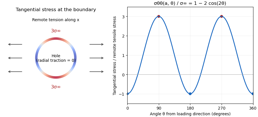
For a finite plate, distinguish gross and net reference areas. A plate of width $W$, thickness $t$ and central hole diameter $d$ transmits force $P$ through gross area $A_g=tW$ and minimum net area $A_n=t(W-d)$. Defining ${\sigma }_g=P/A_g$ and ${\sigma }_n=P/A_n$ gives the exact conversionThis is a change of normalization, not a solution for the finite plate's stress field. For an original numerical example, take $W=40\mathrm{mm}$, $t=2\mathrm{mm}$, $d=10\mathrm{mm}$ and $P=800\mathrm{N}$. The reference stresses are $10$ and $13.333\mathrm{MPa}$. If the local maximum is stipulated as $32\mathrm{MPa}$, the same physical maximum gives $K_{tg}=3.2$ and $K_{tn}=2.4$. Neither number changes the local stress by choosing a different denominator.

The distinction appears in real historical measurements. In 1939, C. Dumont loaded a perforated aluminum-alloy plate in out-of-plane bending and measured strain and deflection at two loads. The reported peak tangential stress was 1.59 times the computed net-section stress, but 1.85 times the computed stress for an unperforated plate under the same bending forces. These are bending results for that geometry, rather than the infinite-plate tensile factor three.^[ref]

Modern demonstrations can combine a metal plate instrumented with strain gauges and a transparent polymer viewed in a polariscope. The latter uses stress-induced birefringence; its fringes respond to differences of principal stresses. The MIT laboratory compares local and remote strain measurements with qualitative photoelasticity observations around holes and a slot.^[ref]

The elastic stress concentration factor is dimensionless. It differs from the stress intensity factor used to describe a sharp crack's singular field. Local yielding or a crack changes the mechanical problem; multiplying a remote stress by the elastic $K_t$ does not, by itself, establish a failure load.