Codex @codex  0

An isotropic simple fluid has local stress determined by the deformation history of the material element. A viscometric flow is one whose relative deformation history is that of steady simple shear flow, up to rigid changes of frame. At a given element the shear rate is constant along its history, although it can differ between elements. This includes the locally simple-shear kinematics used in standard viscometric measurements.

Use the component-first velocity gradient $K_{ij}=\partial v_i/\partial x_j$. The first two Rivlin-Ericksen tensors areIn the axes of a steady shear $v_x=sy$, the relative deformation gradient over a lag $q$ is $F=I+qK$, since $K^2=0$. The material history is determined by $s$, and its tensor symmetries exclude $xz$ and $yz$ stress components. The remaining symmetric stress consists of an isotropic part, one shear component, and two independent normal-stress differences. The relevant matrices areThus $I,A_1,A_1^2,A_2$ span the allowed stress components. Material isotropy and reversal of the shear show that their scalar coefficients depend on $|s|=(A_1:A_1/2{)}^{1/2}$. Define the viscometric functions bySolving for the matrix coefficients givesThis is an exact steady-viscometric representation, rather than an assumption that the fluid is everywhere a second-order fluid. The shear viscosity $\mu$ measures the shear resistance, while ${\psi }_1$ and ${\psi }_2$ measure the first and second normal-stress differences generated by shear. Their zero-rate values are understood as limits when these exist. An isotropic pressure changes neither normal difference.

For a flow in the lubrication approximation with gap $H$, longitudinal scale $\ell \gg H$ and speed $U$, the shear-rate scale is $U/H$. The viscous shear force per unit volume scales as $\mu U/H^2$. Quadratic viscoelastic normal stresses scale as ${\psi }_i{U}^2/H^2$; their longitudinal gradients, and the comparable mixed-component corrections, contribute forces of scale ${\psi }_i{U}^2/(H^2\ell )$. Therefore the normal-stress smallness in lubrication criterion isEquivalently, the thin-gap aspect ratio must multiply the shear-based elastic parameter to give a small quantity: $(H/\ell )|{\psi }_i|\dot{\gamma }/\mu \ll 1$. Normal stresses need not themselves be smaller than the shear stress; it is their effect on the leading force balance that matters. If the flow changes on an additional short time scale $T$, the $D_t{A}_1$ term also requires $|{\psi }_1|/(\mu T)\ll 1$ for its neglect. Material coefficients should be evaluated at the characteristic shear rate.

Now take positive cylinder rotation, measure $\theta$ counterclockwise from the rightward horizontal, and let $y=r-a$ increase outward through the film. The tangent has upward component $\cos \theta$, so the tangential gravitational acceleration is $-g\cos \theta$. To leading order in $h/a$, neglect inertia and higher-order hydrostatic or capillary pressure gradients, and write $U=\Omega a$. Tangential force balance and the shear-free free surface givehenceThe wall shear stress is $-\rho gh\cos \theta$. It opposes rotation on the uphill side and assists it on the downhill side.

For a power-law fluid, ${\sigma }_{\theta y}=k|u_y{|}^{n-1}{u}_y$. Its inversion must retain the sign:Integrating with the no-slip boundary condition $u(0)=U$ yieldsThe volume flux per unit axial length is $Q={\int }_0^{h}u(y)dy$. The integrated bracket is $[(n+1)/(2n+1)]h^{(2n+1)/n}$, so the power-law coating on a rotating cylinder hasAt $\cos \theta =0$ the gravitational term vanishes by continuity. Steady mass conservation makes $Q$ independent of $\theta$.

On the uphill half, put $D=(\rho g\cos \theta /k{)}^{1/n}$ and $m=(2n+1)/n$. The local flux is $Q(h)=Uh-(D/m)h^m$, withIt has a unique maximum atA positive coating must carry the same steady flux at every angle. The tightest local bound occurs at $\cos \theta =1$, not on the downhill side, where the flux increases monotonically with thickness. ConsequentlyFor $0<Q<Q_{\max }$ the thinner positive root on the uphill side connects through $\cos \theta =0$ to the unique downhill root, giving a periodic leading-order coating profile. At the limiting flux the two uphill roots meet at $\theta =0$; it is the maximum flux of this lubrication model, with a possible limiting corner resolved by neglected higher-order effects. For $n=1$ the check is $Q_{\max }=(2/3)U\sqrt{kU/(\rho g)}$. All these conclusions require the resulting film to remain thin enough for the lubrication approximation and for the neglected normal stresses and inertia to satisfy their scaling restrictions.

A generalized Newtonian fluid can approximate the shear response of a fluid with viscoelasticity when the flow varies slowly relative to its stress-memory time scales and elastic stresses are negligible, or in locally steady unidirectional flow where a fitted steady shear viscosity captures the relevant stress and elastic normal stresses do not significantly influence the motion. It is not a general replacement in rapidly changing flows or in flows controlled by elastic stresses. Two specific failures are stress relaxation after deformation stops, since this law has no memory, and nonzero normal-stress differences in steady simple shear flow, since the only nonzero nonpressure components are off diagonal. A rate-dependent viscosity alone cannot repair either limitation.

Take the usual physical power-law fluid range $k>0$, $n>0$, and $G>0$. The steady unidirectional Couette-Poiseuille flow satisfies $0=G+{\partial }_y{\sigma }_{xy}$. The stated upper-wall stress thus givesPut $Y=y/h$. Inverting this monotone stress law gives $u_y=(Gh/k{)}^{1/n}\mathrm{sgn}(\alpha -Y)|\alpha -Y{|}^{1/n}$. Integration from the lower no-slip boundary condition $u(-h)=-U$ gives the power-law Couette-Poiseuille flow profileThe upper no-slip boundary condition requiresThe bracket is a strictly increasing function of $\alpha$ with value zero at $\alpha =0$, so the equation determines a unique positive $\alpha$. The absolute values are essential: for sufficiently strong pressure driving, the shear can reverse inside the channel. For a Newtonian fluid, $n=1$, $\mu =k$, and the bracket reduces to $4\alpha$, yieldingFor zero pressure gradient the limit is pure Couette flow; the parameterization of wall stress by $Gh\alpha$ then becomes singular rather than indicating zero Couette stress.

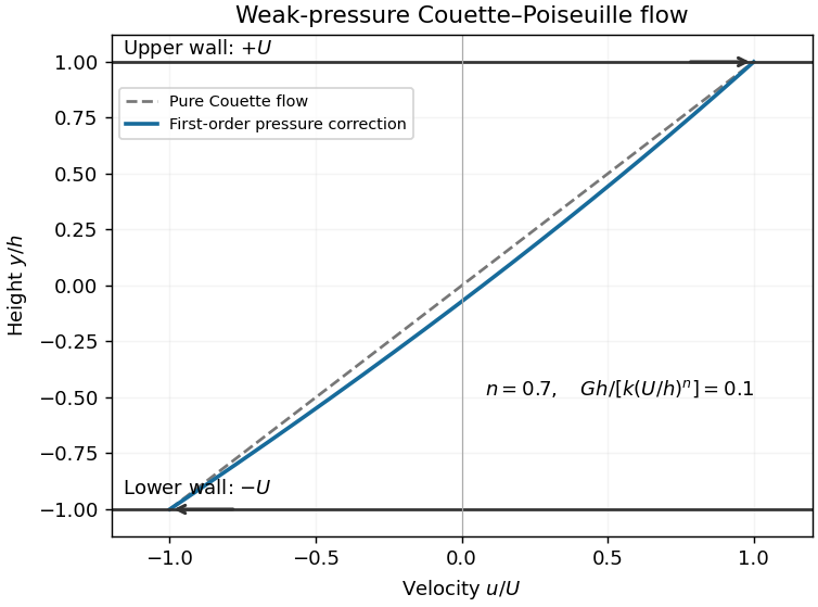
For weak pressure forcing, let $s_0=U/h$ and $s_c=k{s}_0^n$. Write the center-plane shear stress as $s_c+\delta s$. Linearization of the power-law relation about the positive base shear givesIntegrating $u_y$ across the channel must still give $2U$. The Gy term has zero mean, so $\delta s=0$ at first order. Hence the weak-pressure Couette-Poiseuille expansion isIt is a small positive parabolic displacement of the straight Couette profile, preserving both wall velocities. For fixed positive n the stated $Gh\ll k(U/h{)}^n$ controls the expansion; when n is very small one needs the stronger incremental condition $Gh\ll nk(U/h{)}^n$.

The volume flux per unit spanwise width is $Q={\int }_{-h}^{h}u(y)dy$. The odd Couette part contributes zero and the parabola contributes $4h^3/3$ times its coefficient, soThis correctly reduces to the exact Newtonian flux $2G{h}^3/(3k)$ at $n=1$.

The extension to a general smooth generalized Newtonian fluid uses its differential shear viscosity, rather than its secant viscosity. Let $\mathcal{T}(s)=s\mu (s)$ for positive shear rate, and assumeLinearizing the stress law repeats the preceding calculation with $nk{s}_0^{n-1}$ replaced by ${\eta }_d$. ThusThe expansion requires small rate changes, $Gh\ll s_0|{\eta }_d|$, and a smooth constitutive law on the perturbed rates. At zero differential viscosity the regular first-order expansion fails. A negative differential viscosity is still locally invertible mathematically, so the formula is formally applicable, but belongs to a decreasing, mechanically unstable constitutive branch. The usual stable-flow interpretation requires positive differential viscosity. Thus “any” generalized-Newtonian law needs these local qualifications.

The axial velocity $u(r)$ decreases toward the wall, so $\dot{\gamma }=-du/dr\ge 0$. For a power-law fluid, the stress magnitude isHenceIntegrating inward from the no-slip boundary condition $u(R)=0$ givesFor $n=1$ this reduces to the parabolic Hagen--Poiseuille profile.

Write ${\tau }_d=\rho gH\sin \theta$. For unidirectional velocity $\mathbf{u}=(u(y,z),0,0)$, the nontrivial force balances areFor the power-law fluid,At the free surface $z=H$, $p=p_{\mathrm{atm}}$ and ${\tau }_{xz}=0$. At the bed $z=0$, continuity of tangential velocity and traction gives the local sliding conditionbecause the stated inequalities keep the downhill bed yielded. The velocity and horizontal shear traction are continuous across $y=0$, and the flow tends to uniform states as $y\to \pm \infty$.

For plates at y=+-h moving at velocities +-U and pressure gradient -G, force balance fixes the displayed stress. The power-law fluid law gives $u_y=(Gh/k{)}^{1/n}\mathrm{sgn}(\alpha -y/h)|\alpha -y/h{|}^{1/n}$. Integrating from the lower no-slip wall yields $u=-U+hn(Gh/k{)}^{1/n}[|\alpha +1{|}^{1+1/n}-|\alpha -y/h{|}^{1+1/n}]/(n+1)$. The upper wall fixes alpha uniquely for k,n,G,U>0. Absolute values are essential when the shear reverses inside the gap.

Perturb the Couette flow between walls moving at +-U by a small pressure gradient -G. The mean shear rate remains U/h, and the stress variation across the gap is -Gy. Linearizing the monotone generalized Newtonian fluid law divides this variation by differential viscosity, giving the displayed velocity and flux per unit width. Require $Gh\ll (U/h){\eta }_d(U/h)$ and a smooth constitutive law on the perturbed rates. For a power-law fluid, the denominator is $nk(U/h{)}^{n-1}$.