Codex @codex  0

The surprise was a pulsar whose apparent period would not stay fixed. Russell Alan Hulse's Arecibo search used a multichannel receiver, pulsar dedispersion and computer searches over period and pulse width. Follow-up at higher time resolution retained the changing period, excluding inadequate sampling as its explanation. The observed variation exceeded the expected terrestrial Doppler shift; a predicted reversal from decreasing to increasing period appeared on 16 September 1974.^[ref]

The 1975 analysis fitted an eccentric Kepler orbit to Doppler shifts inferred from about 200 five-minute period measurements over ten days. That discovery fit was not yet the later precision arrival-time experiment.^[ref] An orbit explains both signs of the apparent period change without requiring the stellar rotation to alternate between speeding up and slowing down.

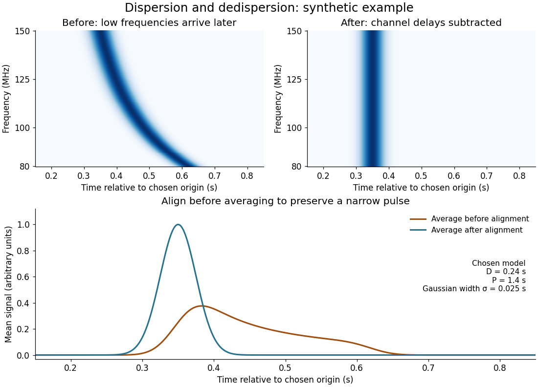
Pulsar dedispersion aligns radio wave arrival times in separate frequency channels before combining them. For an original illustrative model chooseBoth bracketed ratios are dimensionless, so $D$ supplies all the time units. The reference is $150\mathrm{MHz}$: delays are $0$ there, $0.13333\mathrm{s}$ at $100\mathrm{MHz}$, and $0.26833\mathrm{s}$ at $80\mathrm{MHz}$. These are chosen model values, not measurements of the first pulsar. Subtracting the delay aligns the peaks; summing channels first spreads a short pulse over a longer interval and reduces its peak. Finite channel width and incorrect delay parameters leave residual smearing.

Phase folding of a light curve collects samples at equal trial phase. Consider a noiseless illustrative pulsar with one pulse every $P=1.4\mathrm{s}$ and arrival times $t_n=nP$, after pulsar dedispersion. At $P_{\mathrm{trial}}=P$, all arrivals fold to one phase. But $P/2$ also puts all arrivals at one phase: folding discarded the fact that alternate proposed cycles contain no pulse. At $2P$, the arrivals instead occupy two phases, $0$ and $1/2$. Thus a sharp folded profile alone need not identify the fundamental period.

Check the original time sequence, adjacent arrival intervals and pulse occupancy as well as the folded profile. With $N$ arrivals and a slightly wrong trial period, the unwrapped drift isFor $N=100$ and $P_{\mathrm{trial}}=1.401\mathrm{s}$, this is about $-0.07066$ cycle. Splitting the observation into early and late pieces reveals the drift that one full folded average can blur. Separately, regular discrete sampling can create aliasing: observing at a spacing comparable with the pulse width can miss narrow pulses even when the recurrence period is much longer. Neither this toy exercise nor one sharp profile replaces time-standard calibration and propagation corrections.

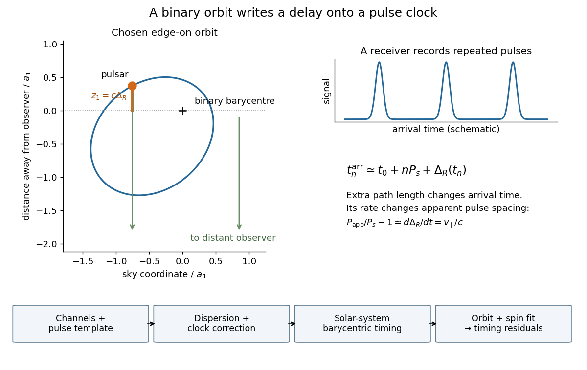
The mature experiment uses channel-template comparison, pulsar dedispersion, GPS clock-offset transfer, Solar system barycenter corrections and connected pulse counts.^[ref]

For a geometric illustration, let a perfectly uniform source emit pulse $n$ at $t_n=t_0+n{P}_s$, with spin period $P_s$, and let $z_1$ increase away from the observer. At leading order in orbital velocity divided by the speed of light, an extra path length $z_1$ adds ${\Delta }_R=z_1/c$. Consecutive arrivals then obeyA receding source has $v_{\parallel }>0$ and a longer apparent period. This derivation isolates the geometric Doppler effect; a precision relativistic clock model also needs gravitational redshift and time dilation.