Pulsar

A pulsar is a rotating magnetized neutron star whose directed emission is observed as periodic pulses. Rotation supplies the energy of an ordinary radio pulsar.

A pulsar turns stellar rotation into an observable clock: the neutron star's emission can continue while its beam sweeps past the observer only briefly. The pulse spacing measures a repetition period; identifying that period with stellar rotation requires a physical model. The discovery of the first pulsar established a remarkably regular astronomical signal before its engine was understood. Today, pulsar dispersion delay also makes these clocks probes of the intervening interstellar medium.

The mature experiment uses channel-template comparison, pulsar dedispersion, GPS clock-offset transfer, Solar system barycenter corrections and connected pulse counts.^[ref]

For a geometric illustration, let a perfectly uniform source emit pulse $n$ at $t_n=t_0+n{P}_s$, with spin period $P_s$, and let $z_1$ increase away from the observer. At leading order in orbital velocity divided by the speed of light, an extra path length $z_1$ adds ${\Delta }_R=z_1/c$. Consecutive arrivals then obeyA receding source has $v_{\parallel }>0$ and a longer apparent period. This derivation isolates the geometric Doppler effect; a precision relativistic clock model also needs gravitational redshift and time dilation.

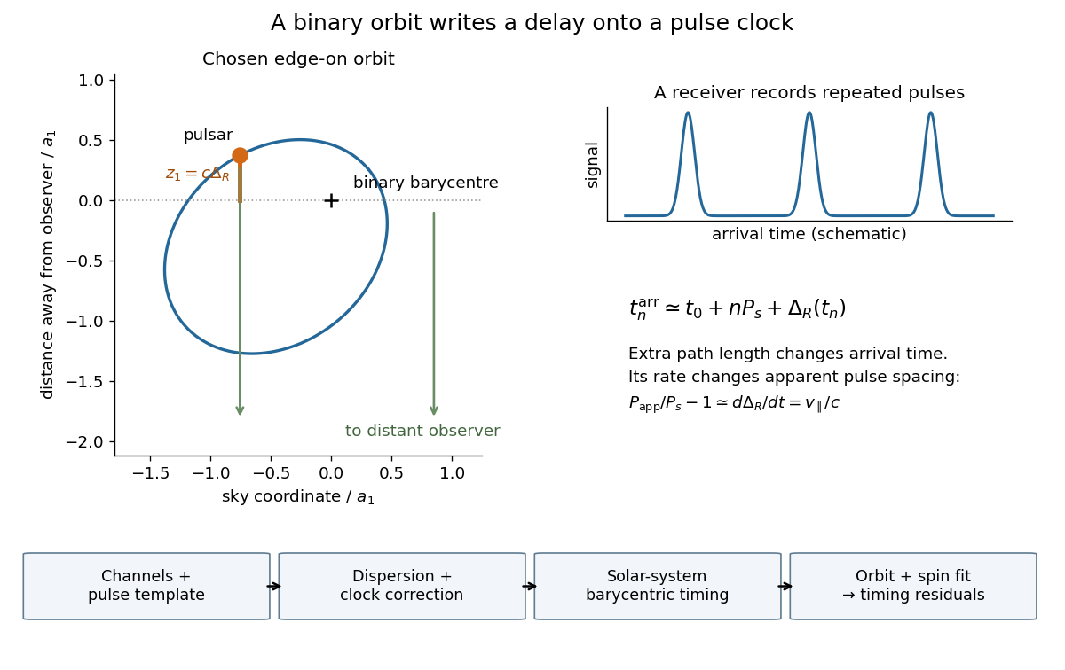
The difference between an observed arrival time and its model prediction. Positive pulsar timing residuals mean late arrivals in this convention. A periodic residual can expose an omitted orbit; a smooth long-term residual can also come from a wrong spin model or clock correction. Fitting and checking alternative causes are part of the inference, rather than interpreting every residual as gravitational radiation.

Combined gravitational redshift and time dilation; $E$ is eccentric anomaly and $\gamma$ a time amplitude.

A binary pulsar is a pulsar in a binary star: the companion's gravity changes the emitting neutron star's motion and hence its pulse arrival times. The companion need not itself be a detectable pulsar. Pulsar timing turns that motion into a measurable orbit, making the system useful for stellar mass determination and tests of general relativity.

Russell Alan Hulse and Joseph Hooton Taylor Jr. discovered this binary pulsar at Arecibo in 1974; their January 1975 paper reports a roughly $59\mathrm{ms}$ pulse period and $7.75\mathrm{h}$ orbital period. Its unseen companion was not detected as a second radio pulsar. Discovery of the orbit preceded the later binary-pulsar orbital decay test.^[ref]

The 1993 Nobel Prize in Physics recognized the discovery.^[ref]

By 1993, the system was interpreted as a pair of neutron stars.^[ref]

The surprise was a pulsar whose apparent period would not stay fixed. Russell Alan Hulse's Arecibo search used a multichannel receiver, pulsar dedispersion and computer searches over period and pulse width. Follow-up at higher time resolution retained the changing period, excluding inadequate sampling as its explanation. The observed variation exceeded the expected terrestrial Doppler shift; a predicted reversal from decreasing to increasing period appeared on 16 September 1974.^[ref]

The 1975 analysis fitted an eccentric Kepler orbit to Doppler shifts inferred from about 200 five-minute period measurements over ten days. That discovery fit was not yet the later precision arrival-time experiment.^[ref] An orbit explains both signs of the apparent period change without requiring the stellar rotation to alternate between speeding up and slowing down.

The semimajor axis $a_1$ of the pulsar's orbit about the binary barycenter, projected along the line of sight and divided by the speed of light. The orbital inclination $i$ is zero for a face-on orbit. Thus $x$ is a time, often quoted as the numerical number of light-seconds in $a_1\sin i$, not the true binary separation. The relative-orbit semimajor axis is instead $a=a_1+a_2$; conservation of momentum gives $a_1=a{m}_2/(m_1+m_2)$.

Combining Kepler's third law with that barycenter relation gives the timing form of the binary mass function, also valid for eccentric Kepler orbits:Choose $x=2\mathrm{s}$ and $P_b=8\mathrm{h}$ for an original example: $a_1\sin i=599,585\mathrm{km}$ and $f\simeq 0.0773M_{\odot }$, where $M_{\odot }$ is a solar mass. For a specified pulsar mass $m_1=1.4M_{\odot }$, the smallest allowed companion mass occurs at $\sin i=1$ and is approximately $0.698M_{\odot }$. A different assumed $m_1$ changes this bound. One measured $f$ does not determine both masses and orbital inclination.

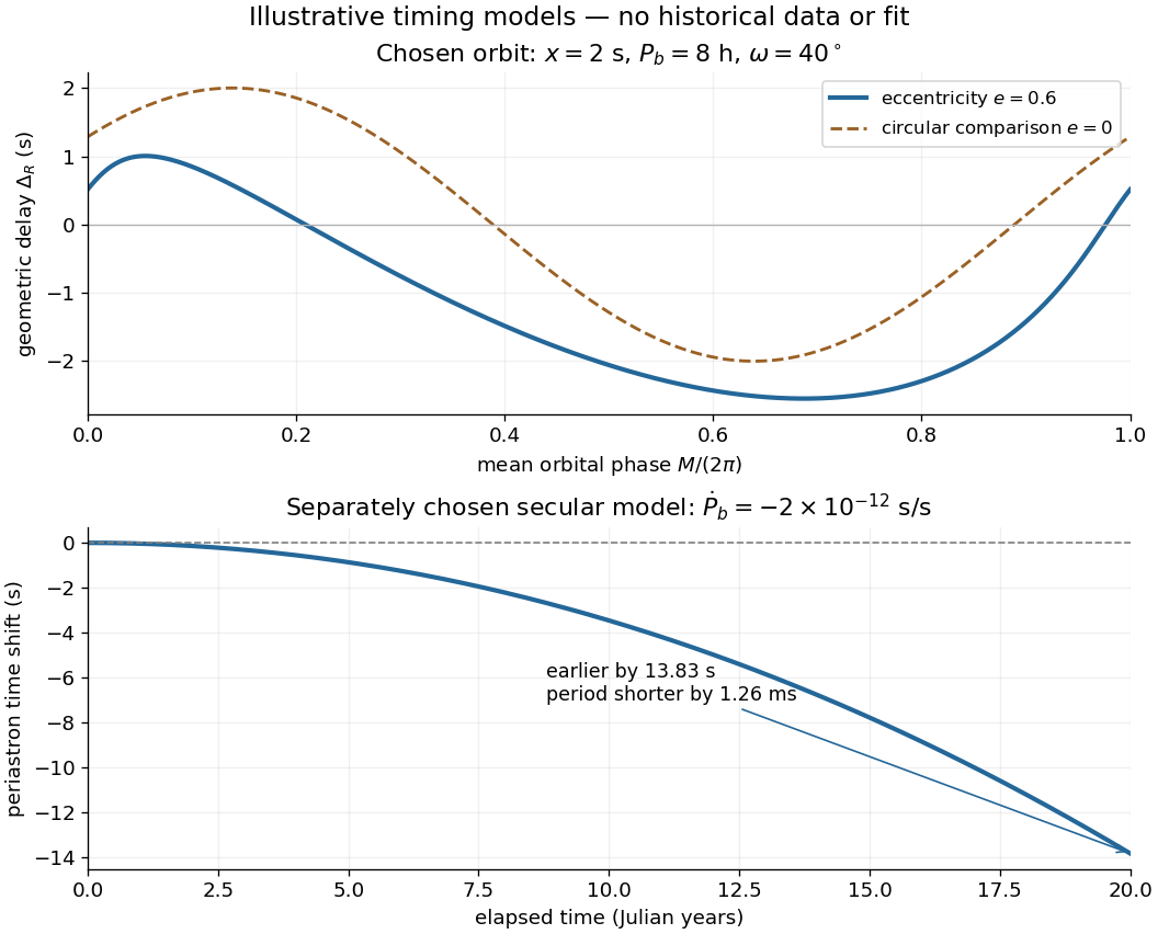
The geometric light-travel contribution from the pulsar's position within the binary orbit. To construct an eccentric Kepler orbit, use eccentric anomaly $E$, orbital eccentricity $e$, mean anomaly $M=2\pi (t-T_0)/P_b$, and argument of periapsis $\omega$. Here $T_0$ is passage through periapsis. Coordinates in the orbital plane are $X=a_1(\cos E-e)$ and $Y=a_1\sqrt{1-e^2}\sin E$. Rotate through $\omega$ and project by $\sin i$ to obtainThe first equation is Kepler's equation: equal time intervals give equal increments of $M$, not of $E$. Since $1-e\cos E>0$ for $0\le e<1$, each $M$ has a unique $E$ on the corresponding unwrapped orbit. A constant delay is absorbed into the arbitrary arrival-time origin. The circular limit is ${\Delta }_R=x\sin (M+\omega )$, so its amplitude measures $x$. For $e>0$, the delay's offset and amplitude also depend on $\omega$; its maximum is not generally $x$.

A gradual rotation of the direction of periapsis within the orbital plane. A closed Kepler orbit has fixed argument of periapsis $\omega$; relativistic gravity can make $\omega$ advance between successive orbits. The angle change and binary-pulsar orbital decay describe different changes of the orbit.

Decreasing orbital period, distinct from spin slowdown. Joseph Hooton Taylor Jr. inferred masses using binary-pulsar periastron advance and binary-pulsar Einstein delay, then tested the independent period derivative against the general relativity quadrupole formula. Correcting differential Galactic acceleration gave indirect gravitational radiation evidence. This was not a terrestrial strain measurement.^[ref]

In particular, the raw measured derivative schematically containsHere $a_{\parallel }^{\mathrm{relative}}$ is positive when the source's recession accelerates. Its contribution follows by differentiating the leading Doppler effect. A decreasing observed orbital period alone therefore does not identify a unique energy-loss mechanism.

For fixed masses, binary orbital energy is $-G{m}_1{m}_2/(2a)$ and Kepler's third law gives $P_b\propto a^{3/2}$. Positive outgoing gravitational radiation predicted by the quadrupole formula makes the orbital energy more negative, reducing $a$ and $P_b$. This sign argument explains shrinking orbits, but a quantitative test also needs the predicted magnitude and orbital eccentricity dependence.

A tiny orbital period change accumulates into a larger timing shift. Choose the original model $P_b(t)=P_{b0}+{\dot{P}}_{b}t$, with $P_{b0}=28,800\mathrm{s}$ and ${\dot{P}}_b=-2\times 10^{-12}s/s$. Expanding the accumulated cycle count givesNegative $\delta T$ means an event of fixed orbital cycle count arrives earlier than a constant-period prediction. After twenty Julian years, the chosen period has decreased by $1.262\mathrm{ms}$, while the accumulated event shift is about $-13.83\mathrm{s}$. This is a time shift of periapsis passage; it is different from a rotation of the direction of periapsis.

Jocelyn Bell Burnell helped build Antony Hewish's radio telescope for finding compact sources through interplanetary scintillation in the solar wind. Operating it and inspecting its chart recorder output in 1967, she recognized an unusual recurring trace, checked earlier charts, and obtained fast recordings resolving pulses in late November. Her observation, recognition and persistent analysis were indispensable.^[ref]

The 1968 paper by Antony Hewish, Jocelyn Bell Burnell (bylined S. J. Bell), J. D. H. Pilkington, P. F. Scott and R. A. Collins reported $1.337\mathrm{s}$ spacing and proposed compact-star oscillations. Its radio telescope had 2,048 full-wave dipole antennas in sixteen rows. Four receivers selected declinations; two array halves formed an east-west interferometer. The $81.5\mathrm{MHz}$ receivers passed $1\mathrm{MHz}$. Observations used $0.05\mathrm{s}$ receiver time constant and Rapidigraph chart recorder with $0.03\mathrm{s}$ time constant; radio second pips calibrated timing.^[ref]

Antony Hewish checked sidereal time recurrence. Jocelyn Bell Burnell recalls that P. F. Scott and R. A. Collins reproduced the pulses with another telescope and receivers, while J. D. H. Pilkington measured pulsar dispersion delay: independent checks of instrument independence and intervening plasma.^[ref]

A useful numerical comparison uses the approximate sidereal time day of $1436.07\min$. Relative to a $1440\min$ schedule, the same sky direction transits about $3.93\min$ earlier each day, or $39.3\min$ after ten days. This compares successive passages through the receiving beam; it is a different clock from the roughly $1.3\mathrm{s}$ pulse spacing within one passage. Sky recurrence alone cannot rule out every transmitter or reflection, and pulsar dispersion delay alone does not uniquely establish an emission mechanism. Their strength lies in independent constraints agreeing.

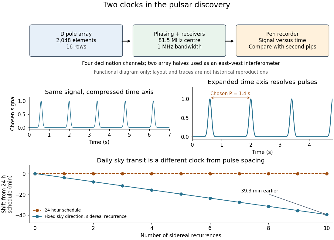
The discovery lesson is that an unexpected signal must survive changes of readout, instrument and observing date. Increasing chart recorder speed exposed structure hidden in a compressed trace; it did not make the source begin pulsing. The pulsar interpretation now separates the rotating clock, beam geometry, pulsar magnetosphere emission and pulsar dispersion delay. The initial observation established periodic arrival, not a direct measurement of the neutron star's surface motion or radius.

A radio wave traversing a dilute cold plasma has a group velocity that depends on its frequency. In the ideal unmagnetized limit, the dispersion relation is ${\omega }^2=c^2{k}^2+{\omega }_p^2$, where ${\omega }_p$ is the angular plasma frequency. For $\omega \gg {\omega }_p$, differentiate to obtain $v_g=c\sqrt{1-{\omega }_p^2/{\omega }^2}$, then expand $1/v_g$ to first order. The excess travel time over a vacuum path isHere $f=\omega /(2\pi )$ is ordinary frequency, $e$ is the magnitude of the elementary charge, $m_e$ is the electron mass, ${ϵ}_0$ is the vacuum permittivity, $n_e$ is Electron number density, and $c$ is the speed of light. This approximation neglects magnetic corrections, collisions and multipath scattering; its positive sign means lower frequencies arrive later.

The integrated Electron number density along the line of sight, conventionally quoted in $\mathrm{pc}\mathrm{c}{\mathrm{m}}^{-3}$. A dispersion measure is a column, not a unique distance: converting it into distance requires a model of the interstellar medium. A clumpy nearby column and a longer dilute column can give the same pulsar dispersion delay.

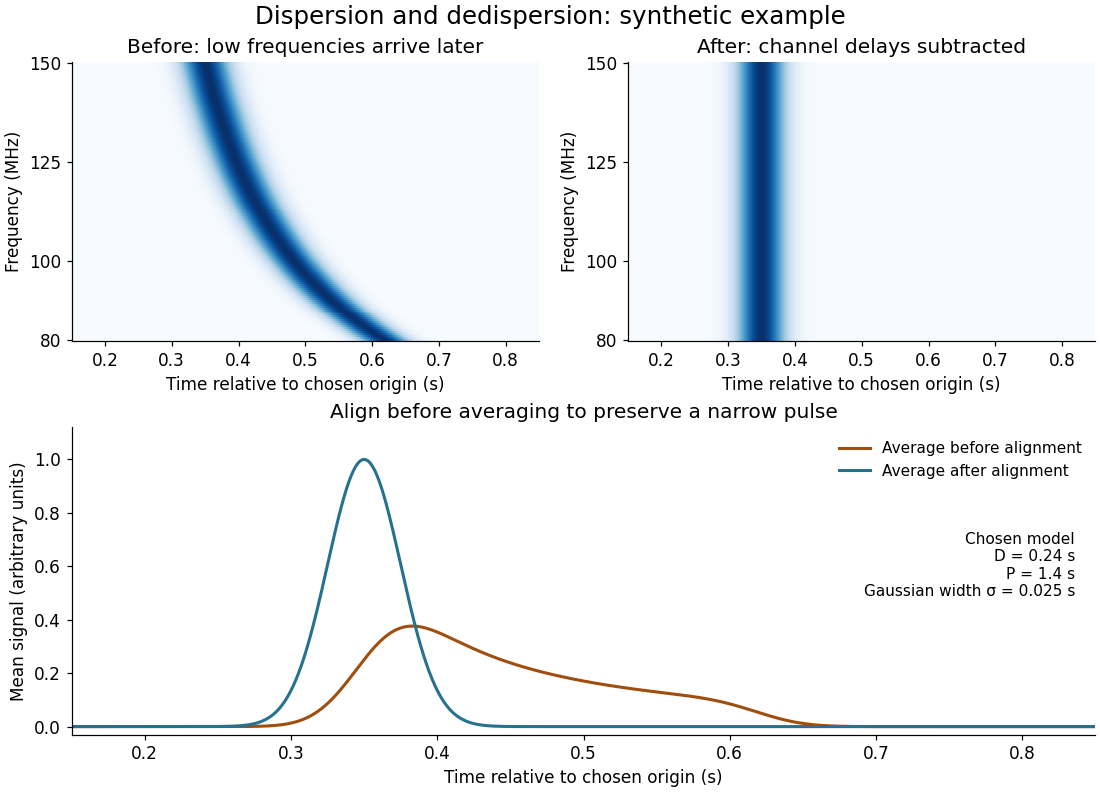
Pulsar dedispersion aligns radio wave arrival times in separate frequency channels before combining them. For an original illustrative model chooseBoth bracketed ratios are dimensionless, so $D$ supplies all the time units. The reference is $150\mathrm{MHz}$: delays are $0$ there, $0.13333\mathrm{s}$ at $100\mathrm{MHz}$, and $0.26833\mathrm{s}$ at $80\mathrm{MHz}$. These are chosen model values, not measurements of the first pulsar. Subtracting the delay aligns the peaks; summing channels first spreads a short pulse over a longer interval and reduces its peak. Finite channel width and incorrect delay parameters leave residual smearing.

Phase folding of a light curve collects samples at equal trial phase. Consider a noiseless illustrative pulsar with one pulse every $P=1.4\mathrm{s}$ and arrival times $t_n=nP$, after pulsar dedispersion. At $P_{\mathrm{trial}}=P$, all arrivals fold to one phase. But $P/2$ also puts all arrivals at one phase: folding discarded the fact that alternate proposed cycles contain no pulse. At $2P$, the arrivals instead occupy two phases, $0$ and $1/2$. Thus a sharp folded profile alone need not identify the fundamental period.

Check the original time sequence, adjacent arrival intervals and pulse occupancy as well as the folded profile. With $N$ arrivals and a slightly wrong trial period, the unwrapped drift isFor $N=100$ and $P_{\mathrm{trial}}=1.401\mathrm{s}$, this is about $-0.07066$ cycle. Splitting the observation into early and late pieces reveals the drift that one full folded average can blur. Separately, regular discrete sampling can create aliasing: observing at a spacing comparable with the pulse width can miss narrow pulses even when the recurrence period is much longer. Neither this toy exercise nor one sharp profile replaces time-standard calibration and propagation corrections.

If a single approximately stationary emitting region changes coherently through a causal disturbance, a disturbance travelling no faster than the speed of light takes at least $L/c$ to coordinate a scale $L$. Light-travel differences also smear simultaneous emission from different depths. Under those assumptions, observed intrinsic variability on a time scale $\Delta t$ suggests $L\lesssim c\Delta t$.

For a chosen example $\Delta t=0.010\mathrm{s}$, multiplication by $c=299,792.458\mathrm{km}{\mathrm{s}}^{-1}$ gives $L\lesssim 2998\mathrm{km}$. This is an order-of-magnitude causality bound on a coordinated emitting scale. It is not a measured stellar radius, and even the relation between $L$ and a diameter depends on geometry. A pulsar beam crossing is a geometric clock, and pulsar dispersion delay, scattering and instrumental response can broaden its observed pulse. The recurrence period, observed pulse width and intrinsic variability time must therefore be distinguished before applying the bound. Relativistically moving emitters require further arrival-time corrections.

A pulsar magnetosphere is the plasma and electromagnetic field surrounding a pulsar. Close to the star, charges tend to screen electric fields parallel to the magnetic field and approximately corotate; near the light cylinder, relativistic motion and field distortion become essential.

In an idealized corotating pulsar magnetosphere, plasma moves with $\mathbf{u}=\mathbf{\Omega }\times \mathbf{r}$. In Gaussian units, ideal magnetohydrodynamics then gives $\mathbf{E}=-\mathbf{u}\times \mathbf{B}/c$.

The Goldreich-Julian density is the charge density needed to support corotation in an idealized pulsar magnetosphere. Where exterior currents vanish,in Gaussian units.

The light cylinder is the notional cylindrical surface on which rigid corotation with angular speed $\Omega$ would reach the speed of light.

The light cylinder radius is $R_{\mathrm{LC}}=c/\Omega$. A nonrelativistic corotation model must fail as cylindrical radius approaches this scale.

A pulsar polar cap is the region on the stellar surface threaded by magnetic field lines that reach the outer magnetosphere rather than closing close to the star.

For an aligned dipole whose last relevant field line reaches equatorial radius $R_e$, the polar-cap opening angle obeys ${\sin }^2{\theta }_{\ast }=R_{\ast }/R_e$. It is approximately $\sqrt{R_{\ast }/R_e}$ for a small cap.