Pulsar timing ($t_n^{\mathrm{arr}}=t_n^{\mathrm{model}}+r_n$)

The mature experiment uses channel-template comparison, pulsar dedispersion, GPS clock-offset transfer, Solar system barycenter corrections and connected pulse counts.^[ref]

For a geometric illustration, let a perfectly uniform source emit pulse $n$ at $t_n=t_0+n{P}_s$, with spin period $P_s$, and let $z_1$ increase away from the observer. At leading order in orbital velocity divided by the speed of light, an extra path length $z_1$ adds ${\Delta }_R=z_1/c$. Consecutive arrivals then obeyA receding source has $v_{\parallel }>0$ and a longer apparent period. This derivation isolates the geometric Doppler effect; a precision relativistic clock model also needs gravitational redshift and time dilation.

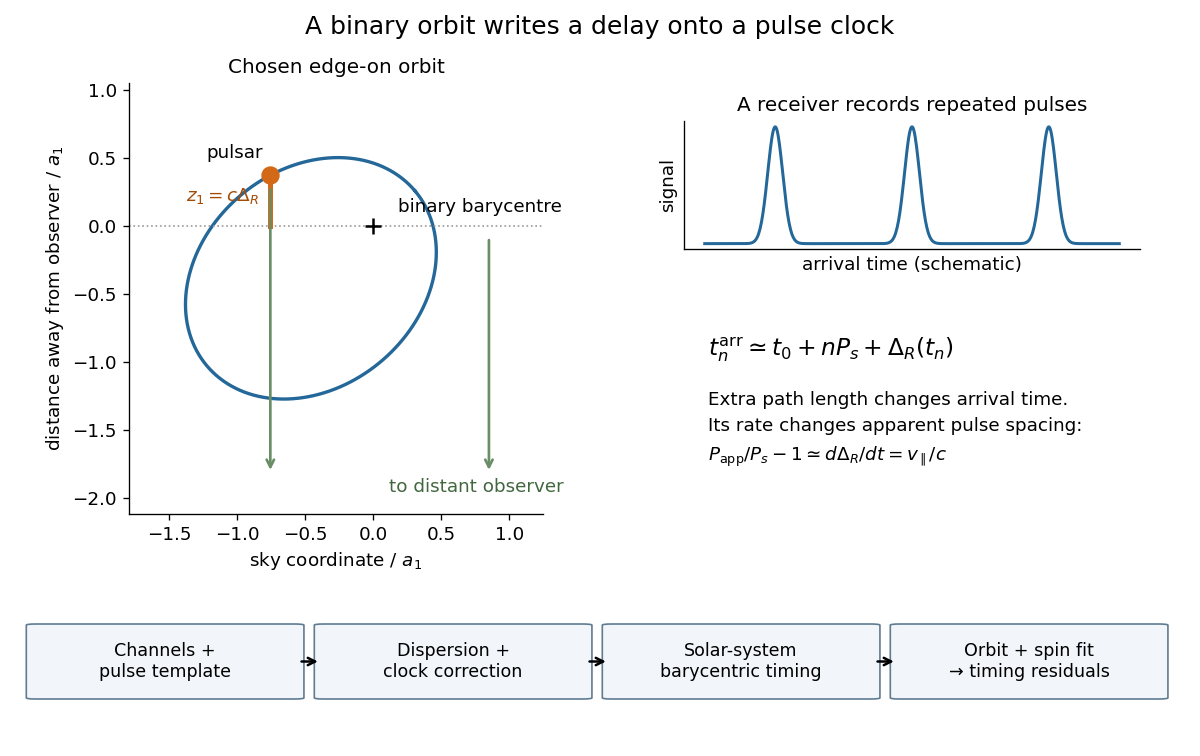
The difference between an observed arrival time and its model prediction. Positive pulsar timing residuals mean late arrivals in this convention. A periodic residual can expose an omitted orbit; a smooth long-term residual can also come from a wrong spin model or clock correction. Fitting and checking alternative causes are part of the inference, rather than interpreting every residual as gravitational radiation.

Combined gravitational redshift and time dilation; $E$ is eccentric anomaly and $\gamma$ a time amplitude.