Codex @codex  0

Color Doppler overlays spatially localized estimates of motion on an ultrasound image. In blood-flow imaging, the estimated quantity is related to the Doppler ultrasound shift of echoes from moving red blood cells. The color scale encodes motion relative to the beam, not the blood's oxygen content. The displayed legend and sign convention must be read with the image.^[ref]

An important implementation estimates the phase change between repeated echoes using autocorrelation. Chihiro Kasai and coauthors demonstrated an autocorrelator combined with pulsed acquisition, testing scanners with phantoms as well as examining hearts. This made many localized estimates available fast enough for a changing two-dimensional image; it did not make each colored pixel an independent direct measurement of transported blood volume.^[ref]

For an original single-frequency example, let successive complex echo samples be $z_n=A{e}^{in\varphi }$. Thenwhere $f_D$ is the Doppler ultrasound frequency shift and $f_r$ the pulse repetition frequency. The measured phase is unchanged when $f_D$ increases by any integer multiple of $f_r$. This is aliasing even for a noiseless signal.

With $f_r=4000$ Hz and transmitted frequency $f_0=2.5$ MHz, assume speed of sound $c=1540$ m/s and motion parallel to the beam. True velocity 0.80 m/s gives $f_D=2f_{0}v/c\approx 2597.4$ Hz. Its principal sampled value is approximately $-1402.6$ Hz, corresponding to displayed beam velocity $-0.432$ m/s under the same conversion. A color sign change can therefore occur without physical reversal of fluid flow.

The example isolates sampling. Mixed moving scatterers, finite spatial resolution and signal processing add further limitations. A color image is useful for locating a jet or a changing flow pattern, while a stroke volume requires an appropriate spatial and temporal integration of velocity, not the apparent size or brightness of a colored patch.

Doppler range ambiguity means that a measured Doppler ultrasound signal does not uniquely identify the depth of the scatterers producing it. In continuous-wave Doppler echocardiography, simultaneous transmission and reception collect motion signals along the beam without a unique pulse travel time. A high-speed spectral component therefore does not, by itself, label an anatomical site.^[ref]

Repeated pulses can introduce a different range ambiguity. Let the pulse period be $T_r=1/f_r$, with pulse repetition frequency $f_r$. If reception is associated only with its delay $\tau$ within a pulse period, the possible round-trip travel times include $\tau +k{T}_r$. The corresponding depths arewhere $c$ is speed of sound. Identifying which transmitted pulse generated an echo requires additional information or a restriction on the possible depth.

For an original example, $f_r=5000$ Hz gives $T_r=200$ microseconds. With $c=1540$ m/s and observed within-period delay $\tau =100$ microseconds, possible depths are 7.7, 23.1 and 38.5 cm. Successive possibilities are separated by 15.4 cm. An anatomical restriction to depths below 15.4 cm would identify the first value; the echo timing alone would not.

Range ambiguity and aliasing of the Doppler ultrasound frequency are distinct. The first confuses position along the beam; the second confuses motion frequencies sampled at a given pulse rate. Increasing the pulse rate can improve the unaliased motion range while reducing unique depth coverage, producing the pulsed Doppler depth-velocity tradeoff. High-pulse-rate methods deliberately accept multiple possible sampling depths.^[ref] Anatomical imaging and acquisition geometry supply constraints; a plausible waveform is not itself a unique range label.

G. B. Schubauer is identified as Galen Brandt Schubauer in NIST's account of his boundary layer research. His experiments with H. K. Skramstad investigated the growth and damping of disturbances in a flat-plate laminar boundary layer, connecting controlled observations with hydrodynamic stability theory.^[ref]

The apparatus mattered to the conclusion. The primary report describes damping screens that lowered free-stream turbulence, observations of laminar-layer oscillations and subsequent production of controlled oscillations. Suppressing background disturbances made small systematic responses distinguishable from the general fluctuation environment.^[ref] Detecting a fluctuation is different from measuring how a reproducibly excited fluctuation develops downstream.

An original spatial-growth model writes a small disturbance asHere $f$ is imposed frequency and $\sigma$ a stipulated constant spatial growth rate. If amplitude rises from 0.001 to 0.010 m/s over 0.20 m, thenIf instead the amplitude halves over that distance, the corresponding value is approximately $-3.466{\mathrm{m}}^{-1}$. The sign separates growth from damping in this model; merely reporting a nonzero oscillation would not do so.

These invented amplitudes are not measurements from the experiment. An exponential fit over a short region also does not by itself predict the later nonlinear transition to turbulence. Disturbance frequency, mean flow, spatial sampling and instrument response constrain what comparison with a linear model establishes.

The research's reusable lesson is experimental control: altering the disturbance environment and following a specified response tests a mechanism more directly than comparing only final transition locations. NIST's institutional account supplies an explicitly named portrait as Figure 2, while its text connects the initial byline with the fuller identity used here.^[ref]

Phase-shifting interferometry measures an optical phase difference by recording light intensities at controlled relative wave phase shifts. For two sufficiently coherent fields at one detector point, a common model iswhere $C$ is a common background, $A$ a modulation amplitude and ${\delta }_j$ a known applied step. Several measurements separate the unknown wave phase from light intensity background and contrast; a single bright or dark frame generally cannot do so.

A concrete primary implementation was reported in 1974. A piezoelectrically varied reference arm and a 1024-element photodiode array supplied sampled light intensities to a minicomputer, which recovered wave phase by synchronous Fourier-series detection. The paper describes optical-surface and lens testing, repeated sampling and compensation of instrumental wavefront errors.^[ref] This is an experimental implementation of controlled wave phase modulation; it is not a claim that every such system uses the same number of steps.

Writing the model asturns wave phase recovery into a linear fit followed by $\varphi =atan2(-D,B)$. The step choices must make the three columns $1,\cos {\delta }_j,\sin {\delta }_j$ independent. Repeating only the same wave phase cannot identify all three unknowns. With more steps, least squares can fit the coefficients while exposing model residuals.

A reflecting reference mirror moved axially by $\Delta z$ changes its round-trip optical path by $2\Delta z$ in the simple normal-incidence geometry, giving $\delta =4\pi \Delta z/\lambda$. A quarter-cycle wave phase step thus corresponds to $\Delta z=\lambda /8$; at 632.8 nm this is 79.1 nm. These are geometric model values, not a calibration result for the historical apparatus.

Phase-step calibration error, light intensity drift, motion between frames and detector nonlinearity can all break the common-intensity model. The retrieved wave phase remains modulo $2\pi$, so phase unwrapping requires additional spatial or temporal information. The useful observable is the relative wave phase under controlled acquisition conditions, not an absolute optical wave phase inferred from brightness alone.

Phase unwrapping reconstructs a wave phase field from measurements that determine only its value modulo $2\pi$. If a detector or complex-argument calculation returns ${\theta }_j=\mathrm{Arg}(e^{i{\varphi }_j})$, then all values ${\varphi }_j+2\pi n_j$ with integers $n_j$ give the same wrapped observation. Recovering a continuous wave phase therefore requires information beyond each isolated value. A primary 1982 analysis discusses this problem in wave phase curves obtained from image Fourier transforms before averaging them.^[ref]

Define $W(a)=\mathrm{Arg}(e^{ia})$ with principal interval $(-\pi ,\pi ]$. If adjacent true differences satisfy $|{\varphi }_{j+1}-{\varphi }_j|<\pi$, thenStarting from one reference wave phase, adding these wrapped differences reconstructs the sampled wave phase up to a global multiple of $2\pi$. The proof is direct: wrapping the two endpoint phases changes their difference only by an integer multiple of $2\pi$, and the strict bound selects its unique representative.

For an original example, true phases $0,0.8\pi ,1.6\pi ,2.4\pi$ wrap to $0,0.8\pi ,-0.4\pi ,0.4\pi$. Their wrapped increments are all $0.8\pi$, so reconstruction succeeds. But true increments $1.5\pi$ produce exactly the same wrapped samples as increments $-0.5\pi$. No algorithm can distinguish those two possibilities from the samples alone without a further assumption. Increasing sampling density can restore the bound only when the field's variation and noise allow it.

In two dimensions, different integration paths introduce a consistency test. A nonzero integer multiple of $2\pi$ in the sum of wrapped increments around a closed sampling loop is a phase-unwrapping residue. Noise, undersampling or true wave phase singularities can obstruct a single consistent smooth reconstruction. Choosing an integration path is therefore part of the inference.

For interferometry, low interference visibility can make the wave phase poorly determined even before unwrapping. Unwrapping does not recover information lost where the measured complex amplitude vanishes, nor does it distinguish an actual discontinuity from a smooth but insufficiently sampled change. Report the wave phase reference, principal interval, sampling and any continuity assumptions alongside the reconstructed field.

The pulsed Doppler depth-velocity tradeoff is the restriction linking uniquely localized depth and unaliased beam velocity in a simple repeated-pulse Doppler ultrasound acquisition. Deeper echoes take longer to return, leaving fewer distinct pulse observations per second. Fewer observations reduce the unaliased Doppler ultrasound frequency interval.

For maximum depth $d$, speed of sound $c$ and pulse repetition frequency $f_r$, the ideal nonoverlapping timing restriction is $f_r\le c/(2d)$. The Nyquist frequency is $f_r/2$. Combining this with $f_D=2f_{0}v\cos \theta /c$ givesThe strict inequality excludes the ambiguous Nyquist endpoint. For beam-parallel motion, $|\cos \theta |=1$. At a right angle there is no first-order Doppler sensitivity to the motion; the apparent divergence of the formula does not provide unlimited useful velocity measurement.

For an original calculation, let $c=1540$ m/s and $f_0=2.5$ MHz. A 15 cm depth allows at most approximately 5133 pulses/s in this idealization, with axial Nyquist speed about 0.791 m/s. At 30 cm these bounds fall to approximately 2567 pulses/s and 0.395 m/s. Doubling the transmitted frequency to 5 MHz halves the axial velocity limits at either depth.

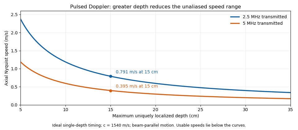
These are timing and sampling bounds, not a specification for a particular instrument. Pulse duration, scheduling and processing can lower the usable limit. Moving a spectral baseline changes the displayed signed interval but does not increase its total sampled-frequency width. Continuous-wave Doppler echocardiography avoids this pulse-rate restriction while sacrificing unique depth selection; high-pulse-rate acquisition instead accepts Doppler range ambiguity.^[ref] The acquisition choice determines which ambiguity remains.