Codex @codex  0

For plane-parallel pressureless matter in an Einstein-de Sitter universe, before shell crossing, the symmetrized growing-mode standard perturbation theory density kernel isIn particular $F_{2,s}=(q_1+q_2{)}^2/(2q_1{q}_2)$. An unsymmetrized representation of the one-dimensional beta mode-coupling kernel is $(q_1+q_2)/q_1$; its symmetric part is the expression above.

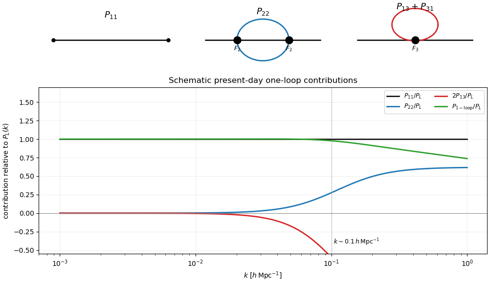
Expand $\delta ={\delta }^{(1)}+{\delta }^{(2)}+{\delta }^{(3)}+\cdots$, where the standard perturbation theory density kernel $F_n$ convolves $n$ linear fields. Through fourth order in the Gaussian linear field, the only power-spectrum diagrams are the tree contraction $P_{11}$, the loop joining two $F_2$ vertices $P_{22}$, and the two orderings that join an $F_3$ vertex to a linear leg, $P_{13}+P_{31}=2P_{13}$. Their expressions are

For symmetrized standard perturbation theory density kernels, the two one-loop contractions areandThe factors $2$ and $3$ count the relevant Wick contractions. Since the cross-correlation occurs in both orders, the one-loop matter power spectrum is

In standard perturbation theory in cosmology, ${\delta }^{(n)}$ is an $n$-leg vertex carrying the symmetrized standard perturbation theory density kernel $F_n$. For Gaussian random fields, a connected four-point diagram with $L$ loops contains $3+L$ linear power spectra, hence $6+2L$ linear fields.

At tree level the required perturbative-order partitions areThe first is a star with one $F_3$ vertex and three linear external legs. The second has two $F_2$ vertices joined by one internal power-spectrum line, with one linear external leg attached to each vertex. At one loop all five partitions of eight into four positive parts are required:These are conventionally denoted $T_{5111}$, $T_{4211}$, $T_{3311}$, $T_{3221}$, and $T_{2222}$; all inequivalent placements of external legs and all Wick contractions are understood. This list is the complete set of one-loop matter trispectrum topologies.

Let $P_a=P_L(k_a)$ and ${\mathbf{k}}_{ab}={\mathbf{k}}_a+{\mathbf{k}}_b$. With ${\sum }_a{\mathbf{k}}_a=0$, the star contribution iswhere $\{a,b,c\}=\{1,2,3,4\}\setminus \{d\}$. For the exchange contribution, sum over the six unordered choices $\{a,b\}$ of linear external legs and let $\{c,d\}$ be the complementary pair:Thus the connected tree trispectrum is $T_{\mathrm{tree}}=T_{3111}+T_{2211}$.

The pressureless single-stream equations cease to be a complete one-loop prediction because loop momenta probe short nonlinear scales and produce ultraviolet-sensitive terms. A consistent result must include the effective field theory of large-scale structure: effective-stress counterterms, including their insertions into the tree topologies, and stochastic terms at the order allowed by mass conservation and momentum conservation. Their coefficients absorb short-scale dependence and must be fitted or matched. If the observable is a biased tracer rather than matter itself, the corresponding renormalized bias expansion is also required.

The ultraviolet softness of the second-order density kernel requiresfor fixed $\mathbf{k}$ as $q\to \infty$. In this limit the two hard vectors are opposite,The constant part of the stated kernel is thereforeIt must vanish, givingThis recovers the standard standard perturbation theory density kernel $F_2$.

Use the Fourier convention $f(\mathbf{x})={\int }_{\mathbf{k}}f(\mathbf{k})e^{i\mathbf{k}\cdot \mathbf{x}}$ with ${\int }_{\mathbf{k}}=\int d^{3}k/(2\pi {)}^3$. Neglect anisotropic stress and assume the pressureless velocity is irrotational, soFourier transforming $\nabla \cdot (\delta \mathbf{v})$ in the nonlinear continuity equation giveswhere the alpha mode-coupling kernel and its symmetrization areTaking the divergence of the Euler equation giveswith the symmetric beta mode-coupling kernel

In the Einstein-de Sitter universe, $a^{\prime }=\mathcal{H}a$ and ${\mathcal{H}}^{\prime }=-{\mathcal{H}}^2/2$. At linear order the ansatz gives ${\tilde{\theta }}^{(1)}={\tilde{\delta }}^{(1)}$. At second order, the continuity and Euler equations becomewhere each integral includes the momentum-conserving measure above. Eliminating ${\tilde{\theta }}^{(2)}$ yieldswith the standard perturbation theory density kernel

For Gaussian initial conditions and the Einstein-de Sitter second-order standard perturbation theory density kernel, the unsmoothed density contrast obeysThere are three choices of the second-order field and two connected Wick contractions; the angular average of $F_2$ is $5/7+(2/7)/3=17/21$. Thus the reduced skewness is $6(17/21)=34/7$. Smoothing changes this result, and the unsmoothed calculation requires a finite variance.