Codex @codex  0

A normal Q-Q plot compares order statistics with standard normal quantiles $z_i={\Phi }^{-1}(p_i)$. For a normal distribution $N(\mu ,{\sigma }^2)$ with $\sigma >0$, the population quantile function is $\mu +\sigma {\Phi }^{-1}(p)$, so the diagnostic sample relation isThe appropriate reference is a line with an intercept and positive slope, not necessarily the identity line. A line can be fitted through two central sample quantiles; R's qqline uses the quantile levels $p=0.25$ and $p=0.75$ by default. Neither that line nor its fitting rule is part of the definition of a normal Q-Q plot. ^[ref]

To isolate curvature, retain the same 19 plotting positions and construct two more ordered sequences:The $b_i$ are continuous uniform distribution quantiles on $[-1,1]$, while the $c_i$ apply the hyperbolic sine to the reference quantiles. Both examples are symmetric about zero. At ranks $1,10,19$, $b_i$ is approximately $-0.947368,0,0.947368$ and $c_i$ is approximately $-1.812618,0,1.812618$. Again, these are constructed values rather than random draws or real data.

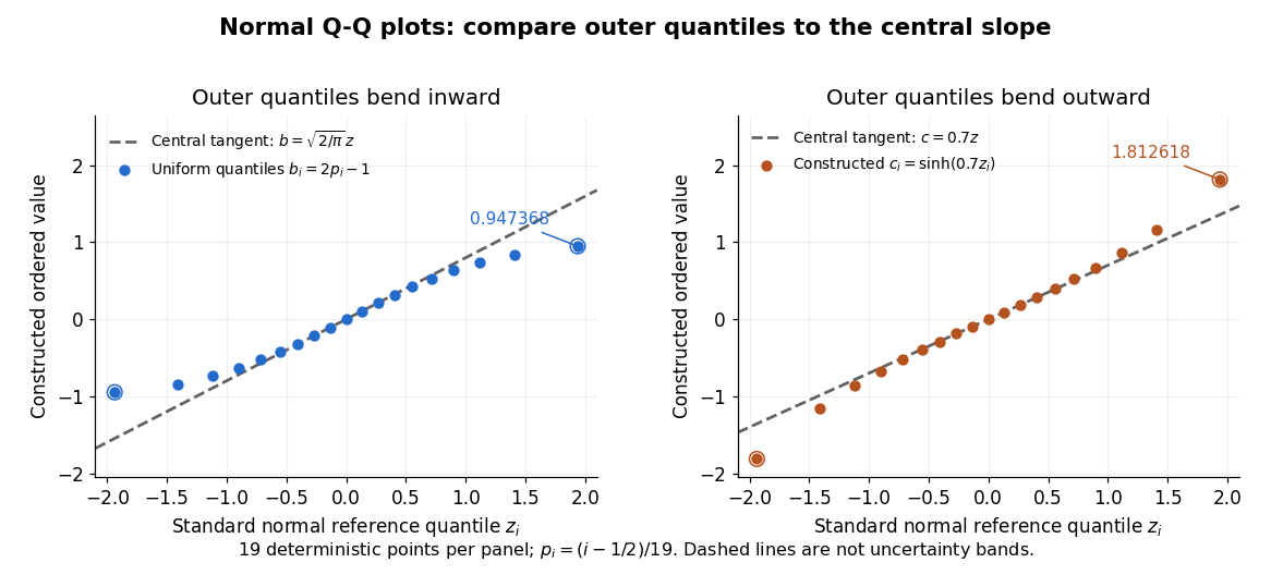
Read these shapes relative to their central slope. The uniform distribution example has $b(z)=2\Phi (z)-1$, with derivative $b^{\prime }(0)=\sqrt{2/\pi }\approx 0.797885$; at the upper endpoint the tangent predicts $1.546246$, while $b_{19}=0.947368$. Its lower end lies above the tangent and its upper end below it: the outer quantiles are compressed. The hyperbolic sine example has $c^{\prime }(0)=0.7$; its tangent predicts $1.356552$ at the upper endpoint, while $c_{19}=1.812618$. Its lower end lies below the tangent and its upper end above it: the outer quantiles are stretched. Unequal departures at the two ends can suggest skewness. The direction of these descriptions assumes that reference quantiles are horizontal and observed values vertical. The graphs illustrate finite-range shape differences; a sample pattern cannot establish an asymptotic tail probability law or membership in a heavy-tailed distribution class.

A nearly straight normal Q-Q plot is a diagnostic, not a proof of a normal distribution or a formal hypothesis test. Random statistical samples fluctuate, particularly at extreme order statistics, and apparent curvature depends on sample size, plotting positions and the reference line. A calibrated hypothesis test or uncertainty band requires its own assumptions and must account for parameters estimated from the same observations. Sorting also discards the original observation order: rearranging a time series leaves its Q-Q plot unchanged, so the plot cannot establish independence.

For a normal linear model, R's diagnostic normal Q-Q plot uses standardized regression residuals, also called internally studentized residuals. ^[ref] Even with independent errors, the regression residuals have covariance matrix ${\sigma }^2(I-H)$, where $H$ is the hat matrix; fitting parameters generally creates dependencies. Dividing by a shared estimated standard deviation creates further dependence, and the distribution of an internally studentized Gaussian residual is not exactly the standard normal distribution. The normal Q-Q plot therefore helps assess error shape alongside other diagnostics rather than certifying independent normal random variables.

Put $G=I-H$. Since $GX=0$, the regression residual vector is $\hat{\epsilon }=G\epsilon$. A linear transformation of a multivariate normal distribution is again multivariate normal, soThis is a singular multivariate normal distribution supported on $\ker X^T$, with dimension $n-p$. In particular,Consequently regression residuals are neither independent nor identically distributed even under the stated model. Their linear constraints include $X^T\hat{\epsilon }=0$, and, if the design matrix contains an intercept, their sum is zero.

Choose an orthonormal basis of the residual space. The coordinates of $G\epsilon$ in that basis are $n-p$ independent $N(0,{\sigma }^2)$ variables, provingFor $n>p$, $s^2$ is an unbiased estimator of ${\sigma }^2$. Orthogonality of $H$ and $G$ gives zero cross-covariance, so the Gaussian fitted and residual vectors are independent. This explains why an appropriate residual-versus-fitted diagnostic has no systematic mean relationship under the model. If $n=p$, no residual information remains for these diagnostics or the variance estimate.

For $h_{ii}<1$, use standardized regression residuals $r_i={\hat{\epsilon }}_i/[s\sqrt{1-h_{ii}}]$ to account for the different residual variances. The diagonal $h_{ii}$ is the regression leverage; $h_{ii}=1$ makes that residual identically zero and cannot be diagnosed by this standardization. With known $\sigma$, the corresponding individually standardized residual has an exact standard normal distribution. With estimated $s$, the internally studentized residual is not exactly normal or a Student t-distribution, and the residuals remain correlated; a normal reference plot is a diagnostic approximation.

Plot the regression residuals or standardized regression residuals against fitted values and each covariate. A persistent curve suggests a misspecified mean, while a fan-shaped spread suggests heteroscedasticity; a scale-location plot helps separate these. A quantile-quantile plot against normal quantiles checks tails, skewness and possible regression outliers. Plot residuals against observation order or time to look for unexplained serial patterns, recognizing that projection already induces the displayed residual covariances. Inspect regression leverage together with Cook's distance for influential observations. Such patterns motivate revising the model; absence of a visible pattern does not prove all its assumptions.

The largest positive regression residual divided by the residual standard error is about $26.6071/5.942=4.48$, $24.7151/5.710=4.33$, and $24.5908/5.737=4.29$ in the three models. In comparison, the most negative regression residual is only about two residual standard errors below zero. At least one observation is much heavier than its fitted value, even after adjusting for sex and height.

A standardized regression residual is $e_i/[s\sqrt{1-h_{ii}}]$, so the regression leverage adjustment can make these ratios larger. The maximum is selected among 100 correlated regression residuals, however; it is not a prespecified single standard-normal observation. These summaries do not give a formal regression outlier test or identify which student is extreme. Ask to check the measurement and data entry, examine residual plots and a normal quantile-quantile plot, and inspect regression leverage and influential observations. A valid observation might reveal a heavier-tailed error distribution, an omitted predictor, or a nonlinear relation. Do not remove it solely because it is unusual, and do not infer from the three summaries alone that all three maxima belong to the same student.

Let $\hat{\beta }=(X^{T}X{)}^{-1}{X}^{T}Y$, $H=X(X^{T}X{)}^{-1}{X}^T$, ${\hat{y}}_i=x_i^T\hat{\beta }$, and $e_i=y_i-{\hat{y}}_i$. The horizontal axis of the residual-versus-fitted plot is ${\hat{y}}_i$, the fitted values, and the vertical axis is $e_i$, the regression residual, in millimetres. Under the normal linear model, $\mathrm{Var}(e_i)={\sigma }^2(1-h_{ii})$, where $h_{ii}$ is the regression leverage.

In the quantile-quantile plot, the vertical values are the ordered standardized regression residualsand the horizontal values are corresponding theoretical quantiles ${\Phi }^{-1}(p_k)$ of the standard normal distribution, with plotting positions such as $p_k=(k-1/2)/n$. The exact plotting-position convention has little practical effect here. Under Gaussian errors these points should approximately follow a straight line; they are not independent because fitting induces residual correlations.

The main visible concern is curvature in the conditional mean. The red smooth in the residual-versus-fitted plot descends from positive residuals at low fitted values, becomes negative in the middle, and rises again at high fitted values. This suggests the strictly linear time effects may be inadequate. There is no clear monotone widening of the residual scatter, so strong heteroscedasticity is not apparent. The quantile-quantile plot has modest tail deviations and a few labelled observations, but does not show a dramatic departure from normality. These plots cannot establish independence across days or laboratories; check residuals against day, laboratory, and sampling order as well. A large coefficient of determination does not remove the visible mean-model concern.

Check that the chosen mean structure adequately describes the transformed response. Examine the residual-versus-fitted plot and residuals versus each predictor: systematic curvature suggests omitted nonlinear effects or an interaction term. Plot residual spread against fitted values, for example using a scale-location plot, to assess homoscedasticity. Compare standardized residuals with a normal distribution using a quantile-quantile plot, especially for finite-sample Student's t-distribution and F-test inference.

Also check independence using the sampling design and residuals versus time, collection site, or other groups; spatially related photovoltaic systems may have correlated errors that are invisible in a residual-versus-fitted plot. Investigate large standardized regression residuals, high regression leverage, and influential observations using Cook's distance. Check that the design matrix has full rank and that severe multicollinearity is not making estimates unstable. Reassess whether the response transformation and retained predictors improve these diagnostics and prediction; a coefficient p-value alone cannot establish model adequacy. If observations are independent only conditional on site effects, use an appropriate dependence model rather than treating correlated systems as independent replicates.

For the residual-versus-fitted plot, compute fitted values ${\hat{y}}_i={\hat{\beta }}_0+{\hat{\beta }}_1{x}_{i1}+{\hat{\beta }}_2{x}_{i2}$ and regression residuals $e_i=y_i-{\hat{y}}_i$; the plotted point is $({\hat{y}}_i,e_i)$.

For the normal Q-Q plot, let $H=X(X^{T}X{)}^{-1}{X}^T$ be the hat matrix for the full three-column design matrix and let $s^2=\mathrm{RSS}/(n-3)$. Form the standardized regression residualsand order them as $r_{(1)}\le \cdots \le r_{(n)}$. R plots $r_{(j)}$ against ${\Phi }^{-1}(p_j)$, where $p_j$ are its plotting positions. For $n>10$, $p_j=(j-1/2)/n$; $\Phi$ is the standard normal distribution function. This standardization is specified in R's diagnostic-plot documentation.

The original PDF shows a residual cloud around zero without compelling systematic curvature or a clear funnel, and a Q-Q pattern approximately following the reference line. Observations 81 and 83 are conspicuous positive tail points, with a smaller lower-tail departure. The plots show no decisive violation of linearity, constant variance or normality, but the extreme residuals merit inspection. They do not test independence across observations and cannot establish that all model assumptions hold.

A regression outlier has a response unusually far from its fitted conditional mean. A standardized regression residual adjusts for regression leverage; an externally studentized residual also estimates noise variance with the observation deleted. Selecting the largest residual among many observations changes its reference distribution. An outlier need not be an influential observation, and unusual valid data should not be discarded solely for being unusual.

A scale-location plot compares the square root of the absolute standardized regression residual with the fitted values. Systematic changes in level or spread suggest heteroscedasticity. It assesses the error scale, while a residual-versus-fitted plot primarily reveals mean patterns as well as changing spread.