Quantile function ($Q(p)=\inf \{x:F(x)\ge p\}$)

The quantile function converts a cumulative probability level into a value. For a cumulative distribution function $F$ and $0<p<1$, use the generalized inverseIt selects the first threshold reaching the requested level. The infimum handles jumps and flat portions, so this construction does not require an ordinary inverse function. Other endpoint conventions are possible at $p=0$ or $p=1$; the open probability interval avoids those issues. NIST introduces the inverse-direction question as the percent point function. ^[ref].

For the finite example under probability distribution,Thus $Q_X(0.1)=0$, $Q_X(0.5)=1$, $Q_X(0.9)=3$. The value at $p=0.2$ is still zero, because $F_X(0)=0.2$ already reaches that level. For $F_Y(y)=y^2$ on $[0,1]$, the quantile function is $Q_Y(p)=\sqrt{p}$, giving $Q_Y(0.5)=1/\sqrt{2}\approx 0.70710678$.

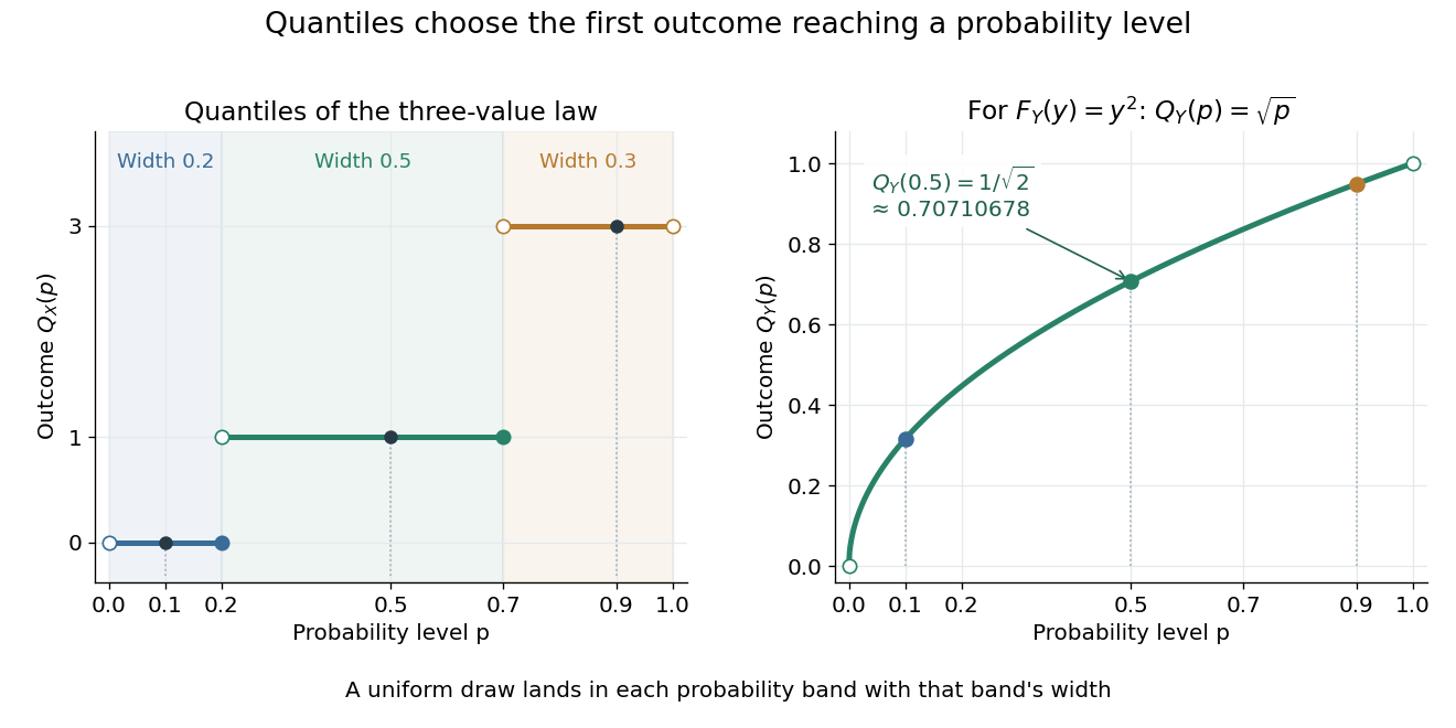
A median is a central threshold; $Q(1/2)$ supplies one, though a median need not be unique. The same quantile function becomes a sampling algorithm through inverse transform sampling. Jumps in $F$ become flat bands in $Q$, precisely the mechanism needed to assign positive probability to one outcome.

For an integrable real random variable with distribution function $F$, the generalized inverse $F^{\leftarrow }(u)=\inf \{x:F(x)\ge u\}$ sends a uniform random variable on $(0,1)$ to the distribution $F$. This follows from $F^{\leftarrow }(u)\le x$ if and only if $u\le F(x)$. Equality of laws proves both the expectation formula and absolute integrability of the quantile. Atoms and flat pieces of $F$ cause no problem.

The $p$-th percentile is a quantile corresponding to cumulative probability $p/100$.

The probable error is the half-width of an interval around a specified central value containing probability $1/2$. For a normal distribution $X\sim N(\mu ,{\sigma }^2)$ with $\sigma >0$, its quantile function giveswhere $\Phi$ is the standard normal cumulative distribution function and $\sigma$ is the standard deviation. The factor is specific to the normal distribution. The centered Cauchy distribution with parameter $\gamma >0$ has probable error $\gamma$, despite having no finite variance. Thus a central probability width need not require a finite second moment.

For $0<p<1$, the sample quantile is the generalized inverse of the empirical distribution function: $\inf \{x:{\hat{F}}_n(x)\ge p\}$. With ordered observations this is $X_{(\lceil np\rceil )}$, including ties. If the population probability density function is continuous and positive at its unique $p$th quantile, the centered quantile has asymptotic variance $p(1-p)/f(F^{-1}(p){)}^2$ under scaling by $\sqrt{n}$.

The quantile function is finite at every probability strictly between zero and one, but need not be finite at one. For any unbounded-above normal distribution, $F(x)<1$ for every real $x$, so its generalized inverse at one is $+\infty$. Inverse transform sampling still produces a real random variable almost surely because a continuous uniform distribution puts zero mass at that endpoint. A real-valued implementation may discard endpoint draws or assign an arbitrary finite value there without changing the sampled law.

For $Q(u)=\inf \{x:F(x)\ge u\}$, $0<u<1$, the quantile function is a monotone function and is left-continuous. The distribution function is right-continuous, giving $Q(u)\le x$ exactly when $u\le F(x)$. If ${\sup }_{v<u}Q(v)<Q(u)$, a point between them has $F(x)<u$ and contradicts this equivalence for some $v\in (F(x),u)$. A jump just to the right of $u$ is possible when $F$ is flat on an interval.

If $q$ is the quantile function of an absolutely continuous probability distribution with probability density function $f$, then $q^{\prime }(u)=1/f(q(u))$ for almost every $u\in (0,1)$. Gaps in the support may give jumps in $q$, so the identity concerns its ordinary almost-everywhere derivative. It follows by differentiating the inverse relation to the cumulative distribution function.

If $U$ has a uniform distribution on $(0,1)$ and $Q$ is the quantile function of a cumulative distribution function $F$, then $Q(U)$ has the desired probability distribution. Indeed, right continuity givesso $\mathbb{P}(Q(U)\le x)=\mathbb{P}(U\le F(x))=F(x)$. This short argument works for both jumps and smooth cumulative distribution functions. MIT's continuous-probability notes introduce the inverse-transformation construction. ^[ref].

For the three-value example, send $U\le 0.2$ to $0$, $0.2<U\le 0.7$ to $1$, and $U>0.7$ to $3$. These intervals have exactly the desired widths $0.2$, $0.5$, $0.3$. For the density example, output $\sqrt{U}$: for $0\le y\le 1$, $\mathbb{P}(\sqrt{U}\le y)=\mathbb{P}(U\le y^2)=y^2$. Independent uniform draws give independent random variables after this deterministic transformation. This direction of construction works even when $F$ has jumps; applying the probability integral transform in the other direction requires its own continuity hypotheses.

For positive mixture weights $w_j$ summing to one, set $C_j={\sum }_{i\le j}{w}_i$ and choose $J=j$ when $C_{j-1}\le U<C_j$, where $U$ has a uniform distribution. Then $V=(U-C_{J-1})/w_J$ has a uniform distribution independently of $J$: for $0\le v\le 1$, $\mathrm{Pr}(J=j,V\le v)=w_{j}v$. This permits exact finite mixture model sampling with a recycled continuous random variable.

If $F_n\to F$ at every continuity point of $F$, then the generalized inverses satisfyat every continuity point of $F^{-1}$. Since a monotone function has only countably many discontinuities, evaluating all quantiles at one uniform random variable gives an almost-sure coupling of the corresponding convergence in distribution.