Topics (374k) Articles (387k) Users (410) Discussions (242) Comments (383) Files (13k) New article

An actual teaching experiment prepares a Kool-Aid stock by weighing powder, transferring it quantitatively into a volumetric flask, and filling to the mark with water. A Genesys 30 spectrophotometer, blanked with water in a cuvette, scans for the peak absorbance wavelength. A Genesys 10 then measures absorbance at that wavelength, with a water reference blank. Each serial dilution transfers of the preceding chemical solution to a volumetric flask and fills to the mark; the protocol records the blank and sample readouts and repeats the halving sequence. These are prescribed experimental steps, not a published numerical data set.[ref]
Quantitative Analysis of Kool-Aid by Mary Jane Simpson. Quantitative Analysis of Kool-Aid by Mary Jane Simpson, Procedure: Prepare Kool-Aid Stock Solution; Measure Peak Absorption of Kool-Aid Solution; Measure Absorbance of Solution at Various Concentrations, steps 1–5
The experiment tests whether absorbance tracks the prepared concentration. Its concentration is powder mass per final volume, so the calibration does not by itself supply a single dye's molar absorption coefficient. The manual identifies loss of discrimination for very concentrated, very dilute, or very similar samples.[ref]
Quantitative Analysis of Kool-Aid by Mary Jane Simpson. Quantitative Analysis of Kool-Aid by Mary Jane Simpson, Background: three limits on distinguishing samples; Procedure: stock preparation and concentration in grams per millilitre
To interpret such a calibration, hold cuvette orientation fixed with its clear faces in the light path, keep fingerprints and bubbles out of that path, and keep the geometric length unchanged. Mix each dilution completely. Re-read the reference blank during the sequence and re-read one standard to test drift. A separate preparation of a standard checks errors propagated through serial dilution; repeating only its instrumental reading does not test the transferred volumes. These controls follow from keeping , , and comparable between readings.
Three mechanisms explain why a straight line can fail. First, scattering of light can divert radiant power away from the photodetector, so cloudiness can raise apparent absorbance without the intended absorbing solute. A reference blank removes only losses shared with the sample. Second, stray light reaching the photodetector can make a strongly absorbing sample appear too transmissive. In an original model with extra detected radiant power in both readings,As the ideal transmittance approaches zero, the reported absorbance approaches for . This finite ceiling is a model prediction, not measured instrument performance.
Third, chemical equilibrium can redistribute the absorbing chemical species when dilution, pH, or temperature changes. Even if each chemical species separately follows the Beer-Lambert law, their combined absorbance is , where is each species' molar concentration; changing those fractions need not preserve one effective molar absorption coefficient. Thus an unknown should be compared with standards under matching chemical solution conditions, within the tested concentration range. A good linear regression alone does not establish chemical selectivity.
Choose an ideal absorbing chemical species with at a fixed wavelength, and a cuvette with geometric length . These are stipulated model parameters. A micromolar molar concentration is , so each additional gives . Five chosen standards therefore predictThe absorbance graph is a straight line of slope , while the transmittance graph shows exponential decay. Equal increments of molar concentration multiply transmittance by ; they do not subtract a fixed transmitted fraction.
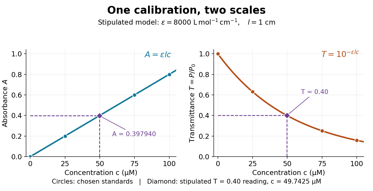
Suppose a measurement returns the stipulated blank-normalized reading under those same conditions. The inferred absorbance and molar concentration areThis lies slightly below the standard because is slightly above . A calibration determined experimentally by linear regression may instead have . Then use , keeping the slope and intercept in their measured units. A nonzero intercept calls for checking the reference blank and sample preparation; it does not uniquely identify the cause.
The decadic molar absorption coefficient specifies absorbance per geometric length and molar concentration. With in centimetres and in , has units ; its SI unit is .[ref]
Beer–Lambert law. IUPAC Compendium of Chemical Terminology, fifth edition (Gold Book) by International Union of Pure and Applied Chemistry; Beer–Lambert law, entry B00626: coefficient name and conventional and SI units
The units cancel in . Since and , one equals . Specify the wavelength and chemical solution conditions when giving a molar absorption coefficient: changing the absorbing chemical species can change it even at fixed total analytical concentration.
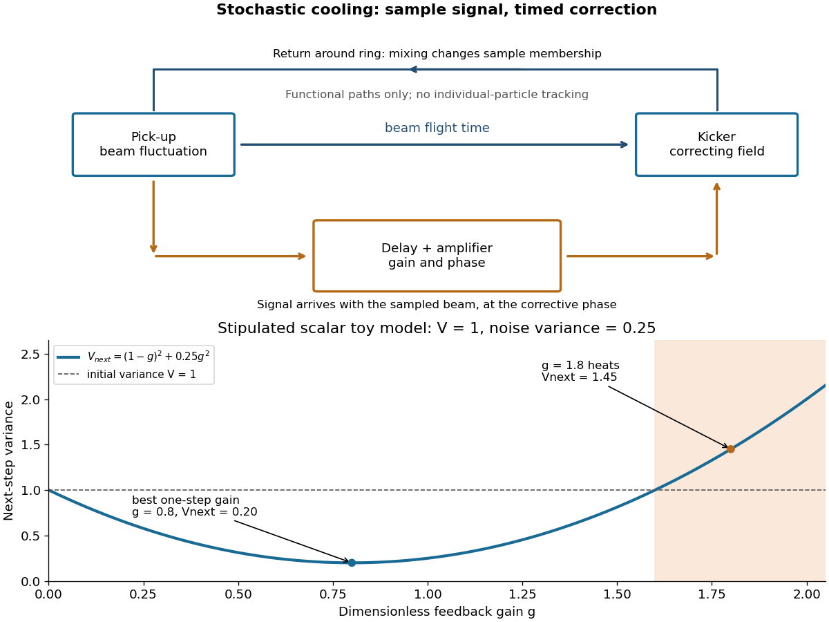
Simon van der Meer's stochastic cooling uses measured beam fluctuations, a pick-up, amplifier and timed kicker. Finite samples supply the signal; other particles and electronic noise contribute unwanted kicks. Delay and oscillation phase must make the correction oppose the sampled deviation.[ref]
This active system dissipates energy; it is no one-particle Maxwell's demon individually tracking antiprotons. The stochastic cooling variance model isolates the tradeoff.
A strong interaction decay must conserve quark flavour and have final rest energy below the initial mass. An excited light baryon can often decay to a lighter baryon plus a pion. A ground-state strange baryon may lack any such open flavour-conserving channel even when its spin permits one. In particular, the Omega baryon cannot decay strongly to a Xi baryon plus a pion because that changes strangeness; its flavour-conserving Xi-kaon channel is closed by the mass threshold. A spin-three-half assignment alone does not imply a strong decay.
A near-surface region whose predominant mobile charge carrier species is opposite to that in the interior: for example a layer rich in electron holes on an n-type semiconductor.
Ordinary solid sodium chloride has the rock salt structure. Choose a conventional cube of side with chlorine anions at the corners and face centers, and sodium cations at the edge centers and cube center. Corner sites are shared by eight cubes, face sites by two and edge sites by four. The unit cell counts are thereforeThere are four formula units per conventional unit cell, rather than four separate NaCl molecules.[ref]
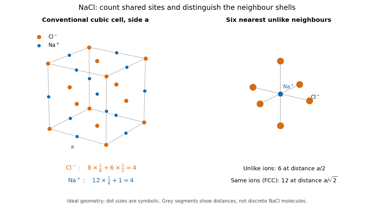
NaCl conventional-cell accounting and the six nearest unlike neighbors
. Original ideal rock salt structure geometry. The left panel includes all boundary sites before sharing is accounted for; the right panel isolates one sodium cation and its six nearest chlorine anions. Grey segments indicate distances, not discrete molecules. Marker sizes do not encode ionic radii. Details.The Bravais lattice is a face-centered cubic lattice. One choice of primitive lattice translation vectors and atomic basis isThe determinant gives a primitive unit cell volume of ; that cell represents one cation and one anion. Four such volumes make the conventional cube. The union of all ion positions resembles a primitive cubic lattice of step only if the chemical labels are discarded: translation by exchanges unlike ions and fails to preserve the chemical structure.
Each ion has six nearest unlike neighbors at distance , along the positive and negative directions of the three cube axes. Thus the coordination number is six. Within either same-species face-centered cubic lattice, the nearest same-ion neighbors instead number twelve: their displacements are permutations of , all of length . Since , those twelve are a more distant shell in the complete sodium chloride structure. The number twelve describes the same-ion FCC lattice neighborhood; six describes the nearest unlike-ion neighborhood.
Fractional crystal coordinates are the dimensionless coefficients in for specified unit cell vectors. They are not Cartesian lengths unless the vectors themselves are included. With primitive vectors, replacing by values differing by integers selects an equivalent position in another unit cell.
In the two-dimensional example under crystal structure, B has position in ordinary length coordinates, but fractional crystal coordinates . Multiplying these coefficients by the two translation vectors recovers the drawn position. Reporting the axes is therefore part of reporting a structure.
Let the net cooling per unit mass of an ideal gas be , with positive constants . At fixed pressure and composition, is constant, so . At a thermal equilibrium , . The specific heat capacity at constant pressure gives . Thus with the displayed growth rate. The equilibrium is stable for , unstable for , and marginal at linear order for . In particular, optically thin Bremsstrahlung with is unstable under this heating law and the isobaric constraint. Fixed-density perturbations have a different criterion.
Pinned article: Introduction to the OurBigBook Project
Welcome to the OurBigBook Project! Our goal is to create the perfect publishing platform for STEM subjects, and get university-level students to write the best free STEM tutorials ever.
Everyone is welcome to create an account and play with the site: ourbigbook.com/go/register. We belive that students themselves can write amazing tutorials, but teachers are welcome too. You can write about anything you want, it doesn't have to be STEM or even educational. Silly test content is very welcome and you won't be penalized in any way. Just keep it legal!
Intro to OurBigBook
. Source. We have two killer features:
- topics: topics group articles by different users with the same title, e.g. here is the topic for the "Fundamental Theorem of Calculus" ourbigbook.com/go/topic/fundamental-theorem-of-calculusArticles of different users are sorted by upvote within each article page. This feature is a bit like:
- a Wikipedia where each user can have their own version of each article
- a Q&A website like Stack Overflow, where multiple people can give their views on a given topic, and the best ones are sorted by upvote. Except you don't need to wait for someone to ask first, and any topic goes, no matter how narrow or broad
This feature makes it possible for readers to find better explanations of any topic created by other writers. And it allows writers to create an explanation in a place that readers might actually find it.
Figure 1. Screenshot of the "Derivative" topic page. View it live at: ourbigbook.com/go/topic/derivativeVideo 2. OurBigBook Web topics demo. Source. - local editing: you can store all your personal knowledge base content locally in a plaintext markup format that can be edited locally and published either:This way you can be sure that even if OurBigBook.com were to go down one day (which we have no plans to do as it is quite cheap to host!), your content will still be perfectly readable as a static site.
- to OurBigBook.com to get awesome multi-user features like topics and likes
- as HTML files to a static website, which you can host yourself for free on many external providers like GitHub Pages, and remain in full control

Figure 2. You can publish local OurBigBook lightweight markup files to either OurBigBook.com or as a static website.
Figure 3. Visual Studio Code extension installation.
Figure 5. . You can also edit articles on the Web editor without installing anything locally. Video 3. Edit locally and publish demo. Source. This shows editing OurBigBook Markup and publishing it using the Visual Studio Code extension. 
- Infinitely deep tables of contents:




All our software is open source and hosted at: github.com/ourbigbook/ourbigbook
Further documentation can be found at: docs.ourbigbook.com
Feel free to reach our to us for any help or suggestions: docs.ourbigbook.com/#contact