Topics (374k) Articles (387k) Users (410) Discussions (242) Comments (383) Files (13k) New article
Consider an ideal gas in chemical equilibrium with homogeneous, identical adsorption sites at fixed temperature. Each intact molecule occupies one site; only one monolayer is allowed. Occupation of distinct sites is independent: neighboring bound molecules do not change binding or release rates. The simplest Langmuir adsorption model has one adsorbing chemical species, no splitting of molecules, and no competitors. Irving Langmuir's 1918 paper treats simple adsorption alongside more complicated cases; its scope exceeds this particular model.[ref]
The Adsorption of Gases on Plane Surfaces of Glass, Mica and Platinum by Irving Langmuir. Langmuir, The Adsorption of Gases on Plane Surfaces of Glass, Mica and Platinum, 1918, theoretical part: Case I and subsequent cases
The derivation is a balance between arrivals finding vacancies and departures from occupied adsorption sites. Let be the arrival-and-binding rate per vacant site and the departure rate per occupied site. Thus has units of inverse pressure per unit time, whereas has units of inverse time. The mean surface coverage obeysAt chemical equilibrium, setting the two terms equal givesThe product is dimensionless. Here is the adsorbing gas's partial pressure, expressed in modern bar, with , and is expressed in . The pascal is the SI unit of pressure. This dimensional is not itself a dimensionless thermodynamic equilibrium constant. A larger gives greater surface coverage at the same and temperature, but does not specify how quickly chemical equilibrium is reached: multiplying both rate coefficients by the same factor leaves unchanged.
Choose , , and as illustrative parameters at one fixed temperature, without assigning a particular material. At , substitution gives, respectively,Solving gives : the three half-occupation pressures are , , and . For , reaching instead requires , or . If the complete-monolayer capacity is stipulated to be , then predicts at . This last number is an original hypothetical example, not a measured uptake.
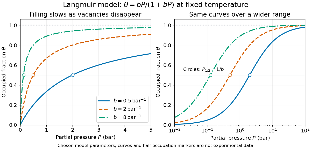
Langmuir isotherms for three chosen values of
. Original model curves at fixed temperature, with in modern bar and , , and . Open circles mark the calculated half-occupation points, not experimental observations. The panels show the same curves on linear and logarithmic pressure axes; the horizontal dashed line marks complete-monolayer capacity. No curve is historical data or a fit to a particular material. Details.The shape follows directly from the finite number of adsorption sites. For , : nearly every arriving molecule finds a vacancy. For , : vacancies become scarce. More formally,Thus surface coverage rises with diminishing slope and approaches one only as . This saturation is a site-capacity limit, not a claim that the gas has reached its condensation pressure. A second layer, different site binding strengths, interactions between bound molecules, or a changing surface invalidate parts of the setup. A good fit alone does not establish identical adsorption sites: a restricted pressure range can hide such differences. The Langmuir adsorption model is useful because it makes the capacity and the pressure scale of filling separate, testable quantities.
For the simple one-solute interface convention, surface excess per molecule is related to the derivative of surface tension with respect to the logarithm of solute activity by the displayed equation. For ideal dilute behavior one may use concentration ratios in place of activity ratios. In molar units, . A local molecular area estimate is . Ionic surfactants can require counterion and activity factors; the simple single-component expression must not be transferred to them without specifying those constraints.
In positional notation with integer base , a carry transfers units in one position into one unit in the next position during addition. Each such transfer lowers the sum of the numeral digits by .
A sonic boom is the sound associated with shock waves from a body moving at a supersonic Mach number. The weak-wave Mach cone describes a propagation geometry rather than the finite pressure signature determining the sound strength.
Ultrasound is sound above the conventional upper limit of human hearing, approximately . In a crystal, ultrasonic travel-time measurements determine long-wavelength elastic wave speeds, which are the small-wavevector slopes of the corresponding acoustic phonon branches.
In the Paschen-Back effect, the external magnetic field interaction becomes large compared with the spin-orbit interaction that holds and coupled. Then ceases to be a good approximate quantum number; become more useful, with leading electronic shifts . In the ideal complete-decoupling limit an electric-dipole interaction preserves , so its spin contribution cancels between the levels and orbital triplet spacing can reappear. Intermediate fields require mixing the coupled states. This is a change of coupling regime, distinct from the weak-field anomalous Zeeman effect; still larger fields require additional terms beyond this linear model.
The anomalous Zeeman effect is Zeeman splitting whose pattern is not the simple orbital triplet. Spin and spin-orbit interaction make the upper and lower Landé g-factors differ. The same weak-field formula still applies when its assumptions hold: “anomalous” does not mean nonlinear in the magnetic field.
For example, take an electronic transition with and , neglecting hyperfine structure. With , the formula above gives and . The two allowed transitions have dimensionless shifts , while the transitions give . Thus there are four frequencies, even though each level contains only two magnetic quantum numbers. This is an independent worked deduction; it should not be substituted for the unresolved widths in the 1896 experiment.
The Landé g-factor is the dimensionless electronic magnetic splitting factor relating a level's magnetic dipole moment to its total angular momentum. In the approximation where total orbital angular momentum and total spin couple to , take the orbital factor as one and the electron spin factor as . For ,This follows by projecting onto and using . At , it gives ; at and , it gives . A level instead has zero first-order electronic shift; the formula's zero denominator must not be used. This is distinct from the statistical weight of an atomic level , sometimes also written .
Viewed perpendicular to the magnetic field, the normal Zeeman effect has a component with linear polarization parallel to the magnetic field and two components polarized perpendicular to it. Along the magnetic field, vanishes and the pair has opposite circular polarizations. Pieter Zeeman described these geometry-dependent patterns in his lecture.[ref]
Light Radiation in a Magnetic Field by Pieter Zeeman. Light Radiation in a Magnetic Field, University of Maryland mirror PDF p. 3, rectilinear/circular oscillator discussion and cadmium photographs
The geometry can be derived from electric dipole radiation. Let the observation unit vector be , with measured from the magnetic field. Radiation retains only the transverse part of the oscillating electric dipole moment :For , take ; its angular light intensity factor is , so it vanishes on axis. For , use normalized complex dipoles . Their angular factors are . Projection gives circles on axis, lines at , and generally elliptical polarization between. These factors assume equal dipole magnitudes; actual line light intensities also depend on initial quantum state populations, transition strengths and collection geometry. No absolute handedness name is needed: it depends on the viewing and phase conventions.
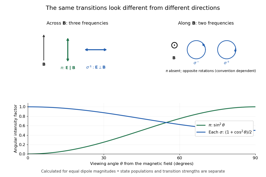
Viewing direction selects the Zeeman polarization pattern
. Original projection diagram with the magnetic field vertical. The top panels show electric-field traces as seen by transverse and axial observers. The lower plot gives calculated dipole angular factors for equal dipole magnitudes; it is not a measured spectrum or an assumption of equal state populations. Details.A transverse polarizer can separate from even before the spectral line components are fully resolved. Along the magnetic field, a quarter-wave plate followed by a polarizer converts the two opposite circular polarizations into distinguishable linear settings. This explains why polarization analysis carried information beyond a small increase in line width.
The normal Zeeman effect is the simple three-frequency pattern obtained in the orbital limit. Assume negligible net spin, negligible hyperfine structure and quadratic shifts, and an allowed electric-dipole interaction between levels with orbital splitting factor one. A level with has only and no first-order shift. For the other levels, gives . Define , rather than the final-minus-initial change of the emitting atom. The electric-dipole selection rule allows , henceMany allowed transitions can share one frequency; a triplet need not mean exactly three transitions. The cleanest illustrative example is , with three upper quantum states and one unshifted lower quantum state. The component is called , and components with this stated convention. During emission the atom changes its magnetic quantum number by .
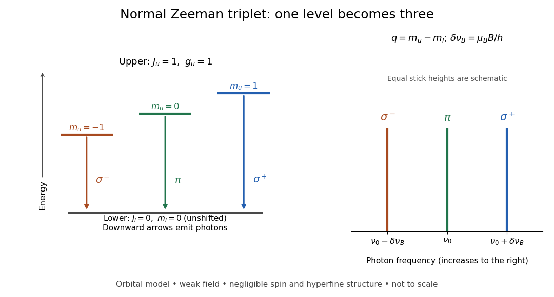
Normal Zeeman triplet from three photon transitions
. Original schematic of the ideal orbital model. The upper splitting factor is one and the lower level has zero first-order shift. Downward arrows show photon emission; the spectrum uses frequency increasing to the right. Equal stick heights are schematic and do not predict observed intensities. Details.For an original numerical example choose and a zero-field vacuum wavelength . Using and gives . The two outer components are separated by . Differentiating the vacuum relation , with the speed of light, givesEach outer component lies about from the centre. Positive means higher frequency and shorter wavelength. Equal spacing in frequency is only approximately equal spacing in wavelength. These are calculated values for a chosen model, not historical measurements.
Use the leading nonrelativistic magnetic coupling for an electronic level with total angular momentum operator , and choose the axis along a uniform external magnetic field , . Write its magnetic quantum number as , so . There are possibilities from to . With Landé g-factor , the first-order shift isHere is the magnitude of the electron electric charge, its mass, the Planck constant, and the Bohr magneton. Both and are dimensionless; with measured in tesla and in joules per tesla, is in joules. The photon frequency shift is in hertz, not angular frequency; indices denote upper and lower levels. NIST states this weak-field convention and its orbital/spin assumptions explicitly.[ref]
12. Zeeman Effect. Atomic Spectroscopy - A Compendium of Basic Ideas, Notation, Data, and Formulas by William C. Martin and Wolfgang Wiese; Atomic Spectroscopy, §12, Eqs. (6)–(8): magnetic-sublevel shift, tesla convention and magnetic splitting factor
The sign follows directly from magnetic dipole potential energy. Within this electronic multiplet, the projected magnetic dipole moment is . Therefore has the displayed positive coefficient. Subtracting the shifts of the two levels and using photon energy gives the transition formula. For the orbital case, gives the same leading frequency spacing as the classical charged oscillator. This explains the historical sensitivity to charge divided by mass; the quantum state derivation here is modern.
“Weak” compares interaction energies: mixing with neighbouring fine structure levels must be small, so remains a useful quantum number. The formula keeps the term linear in and neglects quadratic shifts. It also omits hyperfine structure; if that is resolved and controls the coupling, the appropriate total electronic-plus-nuclear angular momentum and splitting factor must replace . Weak compared with fine structure does not automatically mean weak compared with hyperfine structure.
In August 1896, Pieter Zeeman observed broadened sodium spectral lines at Leiden, initially without resolved components. His lecture describes a slit and concave diffraction grating, then compares the broadening with the sodium doublet separation: about one thirtieth, roughly ångström. This supplied a spectral reference scale, not an absolute magnetic field calibration. Later cadmium photographs displayed resolved transverse triplets and axial doublets.[ref]
Light Radiation in a Magnetic Field by Pieter Zeeman. Pieter Zeeman, Light Radiation in a Magnetic Field, Nobel lecture delivered May 2, 1903; University of Maryland mirror PDF pp. 2–3, paragraphs beginning “In August, 1896”, “The change was however very small” and the cadmium photograph discussion
The fuller report specifies a concave diffraction grating of ten-foot radius with 14,438 lines per inch, an adjustable slit and a micrometer eyepiece with vertical crosswire. Salt in a flame between electromagnet poles supplied the sodium spectral lines. Repeated switching broadened and restored them. To test changes in flame temperature or vapour density, Pieter Zeeman examined photon absorption through a heated porcelain tube with water-cooled glass windows. The arc lamp was displaced from the magnet and its light redirected by a mirror to avoid disturbing the arc. Rotating a narrower tube made the absorption spectral lines equally broad at different heights; the magnetic field still broadened their whole length.[ref]
For the axial test, pierced electromagnet poles let the light travel along the magnetic field. A quarter-wave plate and polarizer selected one broadened edge; rotating the analyser by or reversing the magnet current exchanged the visible edge. The crosswire made its displacement detectable. This tested electromagnetic polarization as well as line width. For its rough estimate the report compared each side's widening with the sodium doublet separation, obtaining about one fortieth, and stated an approximate magnetic field intensity in historical units. These passages give no absolute field-calibration procedure; the inferred charge-to-mass ratio was explicitly a first approximation.[ref]
On the Influence of Magnetism on the Nature of the Light Emitted by a Substance (Part II) by Pieter Zeeman. Pieter Zeeman, On the influence of magnetism on the nature of the light emitted by a substance, Part II, §§14, 20 and 23, printed pp. 10, 16–18; scan is a corrected reprint as its footnote to §24 explains
Hendrik Antoon Lorentz's charged-oscillator theory connected the observed splitting to moving electric charge. In modern language, a line-position measurement needs a wavelength or frequency calibration and an independent magnetic field calibration before it determines a magnetic dipole moment. Resolving the individual components adds the transition information used in the worked example below.
Zeeman populations from an unpolarized angular-momentum multiplet by  Codex 0 Created 2026-10-18 Updated 2026-10-24
An equal incoherent mixture within a fixed total- multiplet has density operator , where is its orthogonal projection. If the applied-field Hamiltonian operator is proportional to and no spin-orbit interaction is retained, its energy eigenstates are the uncoupled states . The Born rule gives their populations by the formula above, or equivalently by squared Clebsch-Gordan decomposition coefficients. Equal populations of coupled states need not give equal populations of magnetic energy eigenvalues.
For , the nonextremal coupled states have weights and in their two uncoupled components. The five dimensionless magnetic energies then have populations ; the zero energy contains two independent states, each with population . In a different, weak-field approximation with a dominant spin-orbit interaction, projecting into the isolated multiplet gives the Landé g-factor spectrum instead. The full operator and its projection must not be interchanged.
Pinned article: Introduction to the OurBigBook Project
Welcome to the OurBigBook Project! Our goal is to create the perfect publishing platform for STEM subjects, and get university-level students to write the best free STEM tutorials ever.
Everyone is welcome to create an account and play with the site: ourbigbook.com/go/register. We belive that students themselves can write amazing tutorials, but teachers are welcome too. You can write about anything you want, it doesn't have to be STEM or even educational. Silly test content is very welcome and you won't be penalized in any way. Just keep it legal!
Intro to OurBigBook
. Source. We have two killer features:
- topics: topics group articles by different users with the same title, e.g. here is the topic for the "Fundamental Theorem of Calculus" ourbigbook.com/go/topic/fundamental-theorem-of-calculusArticles of different users are sorted by upvote within each article page. This feature is a bit like:
- a Wikipedia where each user can have their own version of each article
- a Q&A website like Stack Overflow, where multiple people can give their views on a given topic, and the best ones are sorted by upvote. Except you don't need to wait for someone to ask first, and any topic goes, no matter how narrow or broad
This feature makes it possible for readers to find better explanations of any topic created by other writers. And it allows writers to create an explanation in a place that readers might actually find it.
Figure 1. Screenshot of the "Derivative" topic page. View it live at: ourbigbook.com/go/topic/derivativeVideo 2. OurBigBook Web topics demo. Source. - local editing: you can store all your personal knowledge base content locally in a plaintext markup format that can be edited locally and published either:This way you can be sure that even if OurBigBook.com were to go down one day (which we have no plans to do as it is quite cheap to host!), your content will still be perfectly readable as a static site.
- to OurBigBook.com to get awesome multi-user features like topics and likes
- as HTML files to a static website, which you can host yourself for free on many external providers like GitHub Pages, and remain in full control

Figure 2. You can publish local OurBigBook lightweight markup files to either OurBigBook.com or as a static website.
Figure 3. Visual Studio Code extension installation.
Figure 5. . You can also edit articles on the Web editor without installing anything locally. Video 3. Edit locally and publish demo. Source. This shows editing OurBigBook Markup and publishing it using the Visual Studio Code extension. 
- Infinitely deep tables of contents:




All our software is open source and hosted at: github.com/ourbigbook/ourbigbook
Further documentation can be found at: docs.ourbigbook.com
Feel free to reach our to us for any help or suggestions: docs.ourbigbook.com/#contact