Avogadro constant from sedimentation and diffusion
ID: avogadro-constant-from-sedimentation-and-diffusion

For two observed layers , define the positive logarithmic count slopeSince , where is the molar gas constant, the sedimentation scale height givesSeveral heights check whether one slope fits the whole profile. A mixture of grain radii generally gives a sum of exponential functions, with the larger grains depleted faster aloft; one apparent radius need not describe every height.
An independent readout uses horizontal displacements at lag , avoiding the vertical gravitational drift. Define the one-coordinate mean squared displacement . In a stationary liquid without horizontal advection, translational diffusion predictsA camera sees two horizontal coordinates, so its squared radial displacement has twice the one-coordinate mean. Neither observable is path length or instantaneous velocity. The bulk Stokes–Einstein relation, with dynamic viscosity , then gives
The 1926 lecture compares displacement-based and equilibrium determinations of the Avogadro constant.[ref]
Discontinuous Structure of Matter by Jean Baptiste Perrin. Nobel Lectures, Physics 1922–1941; Discontinuous structure of matter, pp. 152–154
Rotational diffusion supplies a further observable when an identifiable grain orientation can be followed; centre positions alone cannot measure it.
For the chosen model above and , the bulk prediction is . At , and the planar value is . Reconstructing from these stipulated model outputs returns by construction; this arithmetic consistency check is not experimental confirmation. Historical force comes from comparing separately measured profiles and displacements using independently checked material parameters.
The diffusive flux and gravitational particle flux provide another useful connection. With constant drag coefficient , zero vertical net flux readswhere is the downward settling velocity magnitude. With , the chosen model gives . The equilibrium profile forgets how rapidly it was established, while displacement measurements retain that rate information.
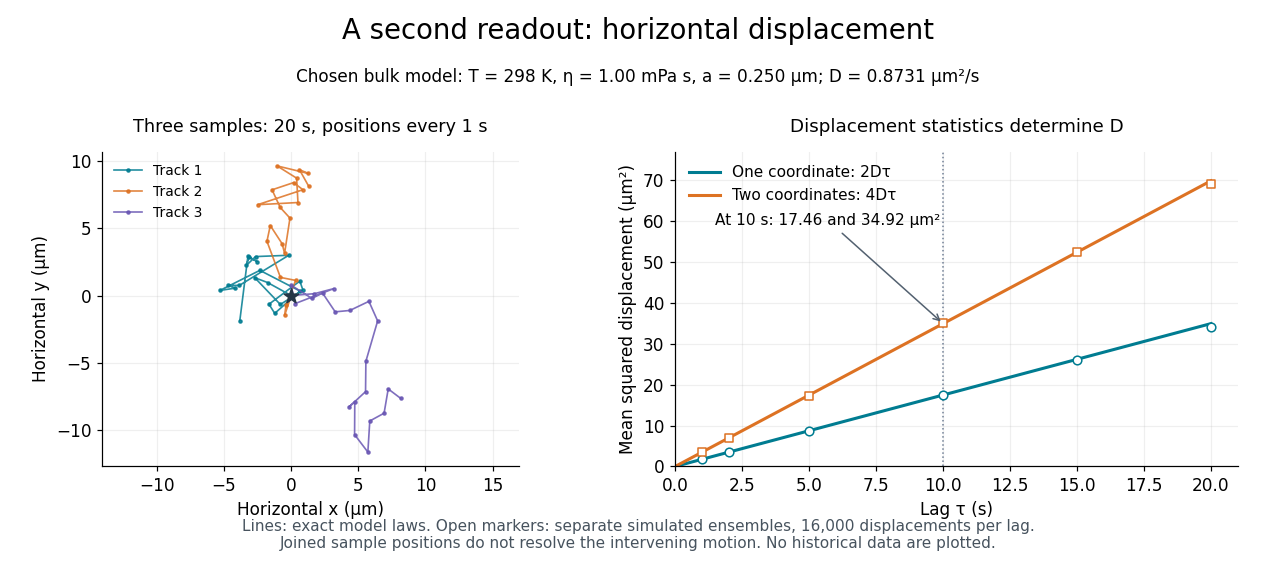
Independent horizontal displacement readout for the chosen Brownian model
. Three simulated planar tracks illustrate sampled endpoints. The other panel compares exact one-coordinate and planar mean squared displacement laws with separate simulated ensembles at each lag. These model observations do not reuse the height counts and are not historical measurements. All use . Details.
New to topics? Read the docs here!