First-order low-pass filter
ID: first-order-low-pass-filter

A first-order low-pass filter with positive constant gain and time constant obeys the ordinary differential equationThe derivative term limits how quickly the plant output follows a changing plant input. A larger time constant means slower adjustment. This standard form, with , is developed in Derek Rowell, MIT 2.004, lecture 20, section 1.1: first-order systems; the following calculation keeps the gain explicit.
Write . The Laplace transform of the derivative is , soSetting the initial condition gives the transfer function . Its single simple pole is , which has negative real part. The unforced response decays, and the input/output map has BIBO stability. The eventual gain for a constant plant input is .
For a unit step, represented by the Heaviside step function , the Laplace transform is . From zero initial condition,Take and , with dimensionless plant input and plant output. Then rises toward . After one time constant, at , it reaches , or of its final value. At , it reaches , or . These percentages describe the rise from zero, rather than an instantaneous jump to the target.
With a nonzero initial condition, the same step instead givesFor and , compare with . Their plant outputs differ by despite having the same transfer function and the same plant input. The extra exponential decay term must be supplied from the initial condition; and alone cannot determine it.
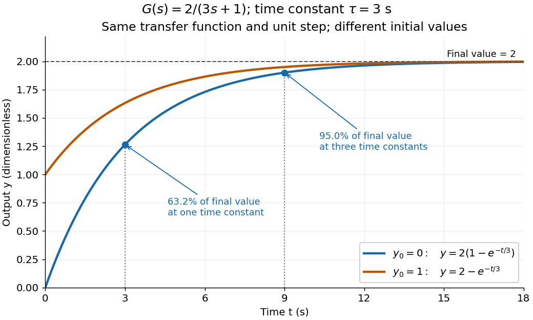
One transfer function, one unit step, two initial conditions
. The first-order low-pass filter has and time constant . The blue curve starts at and the orange curve at . The marked and levels refer to the blue curve's final value ; the two curves' difference is the decaying initial-state contribution. Details.
New to topics? Read the docs here!