A transfer function packages the response of a linear time-invariant system into a rule for turning a plant input into a plant output. Instead of solving a differential equation separately for every signal, take a Laplace transform, multiply by , then transform back. This also makes it possible to compare slow and fast oscillations through the continuous-time frequency response.
Here consider a continuous-time, causal, finite-dimensional linear time-invariant system with one plant input and one plant output . With every initial state set to zero, its transfer function is defined byThe ratio is used where in a common Laplace convergence region; describes the system, independently of that particular plant input. Zero initial state matters: stored motion or another nonzero initial condition can contribute to the plant output even when the plant input vanishes. [ref]
The first-order low-pass filter below shows the same transfer function predicting both a step and a sustained sinusoid. Its pole gives a decay rate, its value at zero gives the eventual gain, and its values along the imaginary axis give the continuous-time frequency response. These descriptions make a useful bridge between a physical relaxation model and control theory calculations.
Substitution into an algebraic transfer function can produce finite amplitude and phase even when the causal system has unstable poles. It then describes a sinusoidal particular solution whose growing homogeneous response is not generically absent. A physically settled frequency response requires transient asymptotic stability; for an unstable causal transfer function, its Laplace region of convergence need not include the imaginary axis.
A first-order low-pass filter with positive constant gain and time constant obeys the ordinary differential equationThe derivative term limits how quickly the plant output follows a changing plant input. A larger time constant means slower adjustment. This standard form, with , is developed in Derek Rowell, MIT 2.004, lecture 20, section 1.1: first-order systems; the following calculation keeps the gain explicit.
Write . The Laplace transform of the derivative is , soSetting the initial condition gives the transfer function . Its single simple pole is , which has negative real part. The unforced response decays, and the input/output map has BIBO stability. The eventual gain for a constant plant input is .
For a unit step, represented by the Heaviside step function , the Laplace transform is . From zero initial condition,Take and , with dimensionless plant input and plant output. Then rises toward . After one time constant, at , it reaches , or of its final value. At , it reaches , or . These percentages describe the rise from zero, rather than an instantaneous jump to the target.
With a nonzero initial condition, the same step instead givesFor and , compare with . Their plant outputs differ by despite having the same transfer function and the same plant input. The extra exponential decay term must be supplied from the initial condition; and alone cannot determine it.
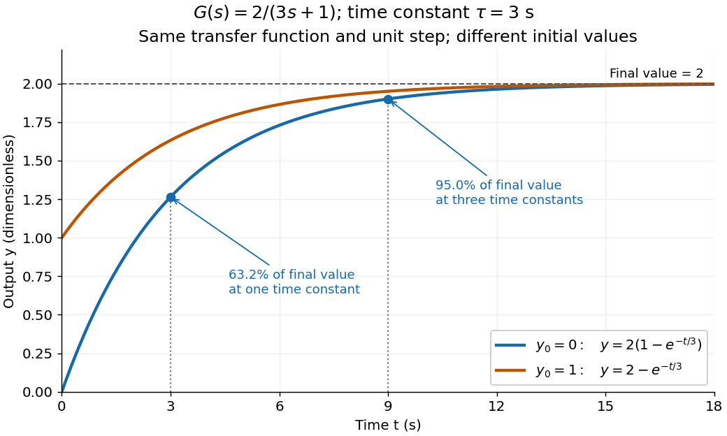
One transfer function, one unit step, two initial conditions
. The first-order low-pass filter has and time constant . The blue curve starts at and the orange curve at . The marked and levels refer to the blue curve's final value ; the two curves' difference is the decaying initial-state contribution. Details.The continuous-time frequency response is the frequency response of a continuous-time linear time-invariant system. From zero initial state, a BIBO stable system driven by a sustained sinusoid approaches the steady responseAny decaying initial or switching transient is separate. The modulus is the amplitude gain; the complex argument is the shift in oscillation phase. Thus evaluating a transfer function at measures both how much of an oscillation passes through and how far it lags.
For the first-order low-pass filter, with , direct complex number arithmetic givesThe phase uses the inverse tangent branch between and . Low angular frequencies have gain close to and little lag. High angular frequencies have gain approximately and lag approaching . This is why the model is a first-order low-pass filter: it suppresses fast variation compared with slow variation. Rowell relates frequency response gain and phase to poles and then introduces Bode plots in MIT 2.004, lecture 32, sections 1 and 2.
At the corner angular frequency,For and , , the gain is , and the lag is degrees. The angular frequency is measured in radians per second; ordinary frequency is measured in hertz (cycles per second), with . Consequently the same corner is , not .
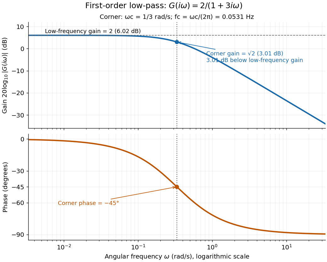
A Bode plot displays the gain and oscillation phase of a frequency response against a logarithmic frequency axis. Gain is often shown as in decibels; phase can use degrees or radians. The first-order low-pass filter loses approximately decibels per factor of ten in angular frequency well above its corner. [ref]
https://www.ocw.mit.edu/courses/2-004-dynamics-and-control-ii-spring-2008/2a0a97261561177bf1a91b07202bb09a_lecture_32.pdf. Rowell, lecture 32, section 2: logarithmic plots
A proper rational transfer function is a rational function whose numerator polynomial has polynomial degree no greater than its denominator polynomial, after common factors are canceled. Every finite-dimensional continuous-time linear time-invariant system of the form , has such a transfer function . [ref]
https://ocw.mit.edu/courses/6-241j-dynamic-systems-and-control-spring-2011/996025f6db0d90b00f11c44fc49b85f9_MIT6_241JS11_textbook.pdf. Dahleh, Dahleh and Verghese, Lectures on Dynamic Systems and Control, section 15.3.1
Bounded-input bounded-output stability means that every bounded plant input produces a bounded plant output from zero initial state. For a causal continuous-time linear time-invariant system with a proper rational transfer function, BIBO stability is equivalent to every pole of the reduced transfer function having strictly negative real part. Cancel common factors first: an apparent denominator root may be absent from the reduced transfer function. For with , the only pole is , so the first-order low-pass filter is BIBO stable. [ref]
https://ocw.mit.edu/courses/6-241j-dynamic-systems-and-control-spring-2011/996025f6db0d90b00f11c44fc49b85f9_MIT6_241JS11_textbook.pdf. Dahleh, Dahleh and Verghese, section 15.3.1 and example 15.5: input/output versus internal stability
Internal asymptotic stability also requires every unforced internal state to decay. A canceled factor can hide a growing internal state. For example, consider the linear system of ordinary differential equationsIts zero-state transfer function can be written and has BIBO stability. Yet from zero initial conditions and a unit-step plant input, grows without bound while the plant output remains bounded. The reduced transfer function conceals that second state. Even a transfer function with no visible cancellations can be implemented with additional hidden states; its poles alone do not establish internal asymptotic stability of an arbitrary implementation.
An input-output gain bounds how large a system's output can be relative to its input, after the input and output measures have been specified. For a zero-initial-state operator and chosen signal norms, its induced signal gain isA finite gain gives . The supremum is over the admissible input class, not merely a collection of trial inputs. Initial-state response must be treated separately.
For an original scalar linear time-invariant system, letUsing the time-domain L-infinity norm, the convolution solution obeysA constant input of suitable sign approaches the limiting ratio , so this bound is sharp. At and , the peak-amplitude gain is1.5: an input bounded by2 gives output bounded by3 from zero initial state, and the constant input approaches that value.
The signal norms change the problem. For the same stable scalar system, the peak frequency response magnitude isIt coincides numerically with the preceding gain in this example. For stable linear systems, this frequency-domain quantity is the energy-signal induced gain associated with the time-domain L2 norm; it should not generally be identified with the peak-amplitude induced gain. MathWorks's linear-model
norm documentation distinguishes this peak frequency-response quantity from its separate impulse-response norm.[ref]The units matter as well: a gain from force input to displacement output has physical units, whereas identical normalized signal units can produce a dimensionless gain. In robust performance, the bound must hold across the allowed control model uncertainty. A nominal gain calculation alone supplies no such universal guarantee.
An induced signal gain is the smallest norm-based amplification bound obtained by taking the worst case over admissible inputs. For a zero-initial-state operator satisfying ,For a linear map this is an operator norm between the specified normed spaces. Axler's definition takes the supremum of output norm over inputs of norm at most1, which is equivalent by linear scaling.[ref]
Linear Algebra Done Right by Sheldon Axler (4th edition). §7F, norm characterization7.88, printedp282
The norms are part of the definition. An original finite-dimensional example usesWith the same maximum-component norm at input and output, , and attains the ratio2. With the Euclidean norm, the Cauchy-Schwarz inequality gives , with equality at . With the sum-of-absolute-components norm, , and attains ratio1. The same matrix therefore has induced gains2, and1 under these three conventions.
For a time-dependent signal, the choice may additionally compare peak amplitudes or integrated squared amplitudes. The example in input-output gain derives a sharp peak-amplitude bound for a scalar dynamic system. A large response to one trial input supplies a lower bound on induced gain; proving a universal upper bound requires controlling every admissible input.
Compatible induced bounds compose. If and , thenThe intermediate norms must be the same. This inequality bounds a cascade without requiring the inputs that maximize the individual blocks to be simultaneously realizable, so the product need not be sharp. In robust performance, both the signal norms and the allowed control model uncertainty must be stated before such a bound can be interpreted.
The Nyquist stability criterion applies the argument principle to a specified negative-feedback return ratio . Assume a proper rational loop with a well-posed interconnection, no poles or closed-loop characteristic zeros on the imaginary axis, and no singularity at the closing part of the contour. Let count poles of in the open right half-plane and let count zeros of there, both with multiplicity. For a positively oriented contour enclosing that half-plane, let be the signed counterclockwise winding of its image under around . ThenA clockwise contour convention reverses the sign of , so the orientation must accompany the formula. Closed-loop input-output stability requires and exclusion of imaginary-axis zeros; simply passing through or encircling is not a conclusion without the pole count and convention.
Poles on the imaginary axis require an indented contour and a corresponding boundary analysis. Also, cancellations in a reduced transfer function can conceal unstable internal states, so a Nyquist conclusion about alone does not prove internal stability of an arbitrary nonminimal realization. The bounded-input bounded-output stability example exhibits that distinction.
The plant output caused by a persistent step change in the plant input, with an explicitly specified initial condition.
Articles by others on the same topic



A transfer function is a mathematical representation used in control theory and signal processing to describe the relationship between the input and output of a linear time-invariant (LTI) system in the frequency domain. It is typically expressed as a ratio of two polynomials.