Holographic wavefront reconstruction
ID: holographic-wavefront-reconstruction

Take stationary scalar monochromatic waves of the same frequency and polarization of an electromagnetic wave, with time convention . Write their complex amplitudes at the recording plane as and , absorbing the common conversion to irradiance into the units. An exposure short enough to avoid fringe motion but long compared with an optical period recordsThe two cross terms are where relative wave phase enters the measured light intensity. Blocking the holographic reference wave leaves and removes them. Loss of mutual optical coherence, incompatible polarization of an electromagnetic wave or motion that averages the relative wave phase similarly reduces fringe contrast. These are useful controls for distinguishing a hologram from an ordinary brightness record. One local cosine value does not uniquely determine a wave phase; known reference structure and separation of the cross terms supply the additional information in the example below.
Model a thin weakly modulated recording by its amplitude transmittanceHere and are real constants in a local linear response to exposure at a fixed exposure time. They describe a chosen amplitude modulation model, not a universal photographic response; an absorbing negative may have . Keep for this passive real-transmission model. Ignore material thickness, saturation, shrinking, clipping and changes of wavelength. Illuminating the processed record with the original gives, immediately after the plate,This follows by multiplying the preceding identity by ; no wave phase detector has been assumed. If is uniform, the desired term reproduces up to a constant. A nonuniform weights the recovered field. With a strong holographic reference wave, the contamination is small relative to , but it is retained in this identity. Subsequent diffraction propagates each term: reproduction at the plate is the starting boundary field, not yet a focused image.
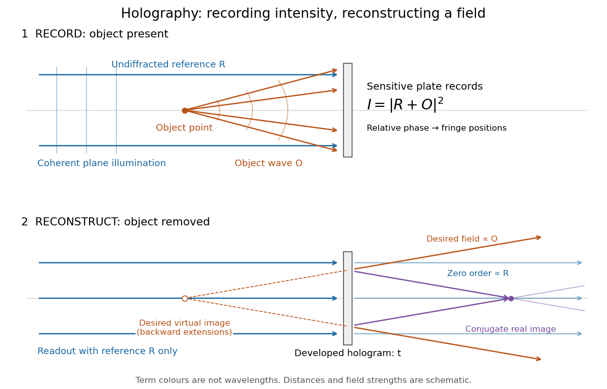
Recording light intensity and reconstructing wavefronts: original functional geometry for in-line holography
. Details. 
The schematic uses a plane wave reference and one optical point source to separate the functions. The top row records ; the bottom removes the object and illuminates the developed hologram with . Dashed extensions identify the desired virtual image; the conjugate component converges toward a real image. All three outgoing components coexist. The coloured paths distinguish terms, not different wavelengths; distances and strengths are schematic. This functional drawing is not a reconstruction of the historical apparatus.
New to topics? Read the docs here!