 Lamb shift line-centre model

Consider an original illustrative resonance model, with all numerical settings chosen here. On one isolated branch approximate the transition frequency by $\nu (B)={\nu }_0+aB$, with known slope $a=20MHz/mT$ and drive frequency ${\nu }_d=1300\mathrm{MHz}$. Choose ${\nu }_0=1100\mathrm{MHz}$, hence resonance field $B_r=10\mathrm{mT}$. This local linear model omits hyperfine structure and nonlinear level mixing; it is not the historical hydrogen Zeeman splitting calculation.

Use a Lorentzian line shape for a weak-drive current dip,Choose baseline $C=1$, depth $A=0.25$ in arbitrary detector signal units, and full width at half maximum $w_{\nu }=100\mathrm{MHz}$, so $w_B=5\mathrm{mT}$. The half-depth points are $B_r\pm w_B/2$; this checks the factor of four. If an exponential decay with lifetime $\tau$ alone set this width, natural linewidth would give $w_{\nu }=1/(2\pi \tau )$ and $\tau \simeq 1.59\mathrm{ns}$. The chosen width is an explanatory input, not a measurement of a historical lifetime.

Generate 65 equally spaced fields from $2$ to $18\mathrm{mT}$ and add independent Gaussian noise with known standard deviation ${\sigma }_I=0.004$ signal units. A simultaneous nonlinear regression fit of $C,A,B_r,w_B$ gives $B_r\simeq 10.0007\mathrm{mT}$, $w_B\simeq 4.9305\mathrm{mT}$ and ${\nu }_0\simeq 1099.986\mathrm{MHz}$. With residual derivatives $J_{ik}=\partial I(B_i)/\partial {\theta }_k$ and $\theta =(C,A,B_r,w_B)$, the local covariance matrix estimate isIt gives centre standard deviation $0.01427\mathrm{mT}$, or $0.285\mathrm{MHz}$ in the inferred intercept. This uses the stipulated noise variance and a local linear approximation, rather than treating the width as the centre error. Repeated noisy samples can locate a broad line's centre much more closely than its width.

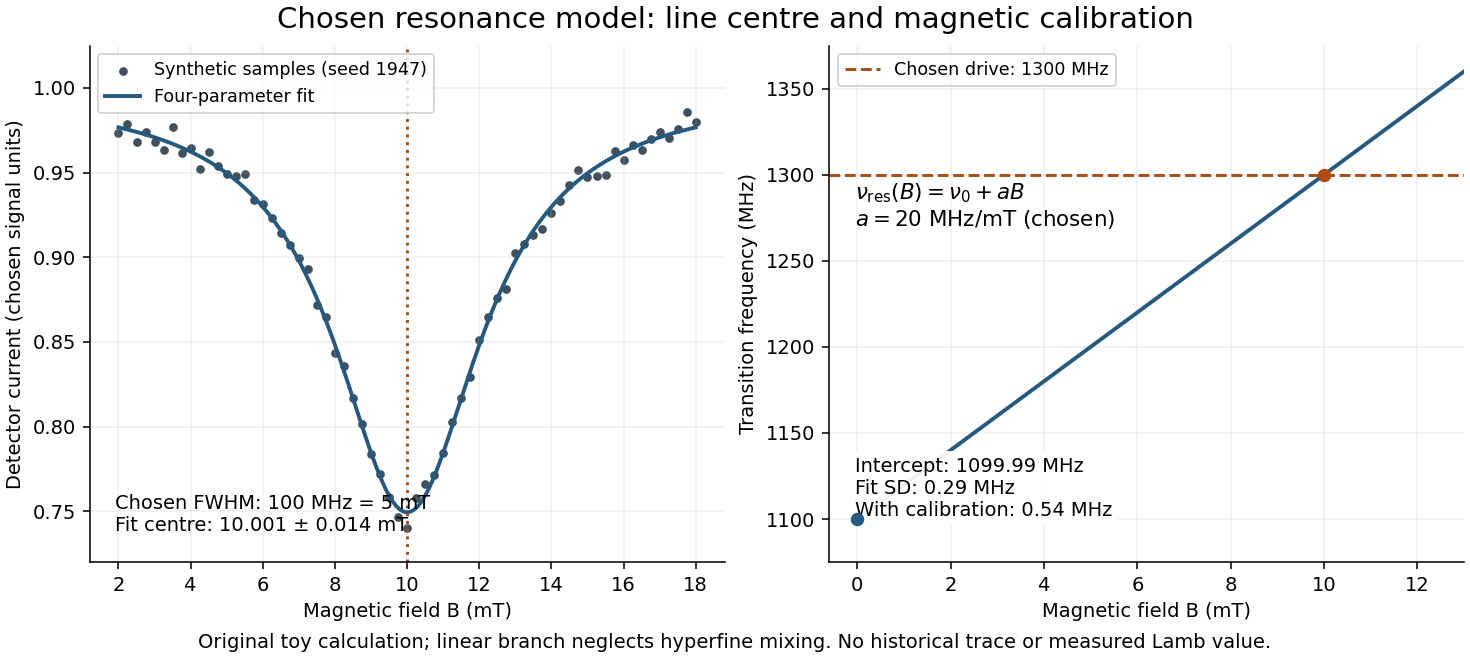
Include a common magnetic calibration offset with standard deviation $u_b=0.020\mathrm{mT}$, a fractional gain error $u_g=0.001$, and independent drive-frequency error $u_d=0.100\mathrm{MHz}$. To first order the inferred variance isHere $u$ denotes a standard uncertainty, not a frequency. The four contributions in $\mathrm{MHz}$ are $0.285$, $0.400$, $0.200$, and $0.100$; adding their squares gives $u({\nu }_0)\simeq 0.540\mathrm{MHz}$. The calibration offset shifts all sampled fields together, so increasing the sample count cannot average it away. Uncertainty in $a$, unresolved components, asymmetric line distortion, and errors in the assumed field dependence would require additional terms or a richer model. The historical inference requires the appropriate Zeeman splitting branches, rather than simply drawing a straight line through one resonance.