Zeeman splitting is the separation of energy levels or mode frequencies by a background magnetic field. In atomic physics, the magnetic field couples to a magnetic dipole moment, lifting quantum degeneracy. Transitions between the shifted quantum states can turn one spectral line into several. A split level and a split spectral line are different objects: the emitted photon measures the difference between two level energies, and the electric-dipole selection rule determines which differences appear.
The Stern-Gerlach experiment also probes magnetic dipole moments, through beam deflection in a magnetic field gradient. Here the readout is a spectral line.
The pattern makes an invisible magnetic field visible through spectroscopy. It also reveals angular momentum and magnetic dipole moments inside chemical atoms. Zeeman slowers exploit a changing resonance frequency to keep moving chemical atoms absorbing laser photons; a magneto-optical trap combines position-dependent shifts with electromagnetic polarization and laser cooling. Related mode shifts occur in Zeeman splitting of an antiferromagnetic spin wave.
An equal incoherent mixture within a fixed total- multiplet has density operator , where is its orthogonal projection. If the applied-field Hamiltonian operator is proportional to and no spin-orbit interaction is retained, its energy eigenstates are the uncoupled states . The Born rule gives their populations by the formula above, or equivalently by squared Clebsch-Gordan decomposition coefficients. Equal populations of coupled states need not give equal populations of magnetic energy eigenvalues.
For , the nonextremal coupled states have weights and in their two uncoupled components. The five dimensionless magnetic energies then have populations ; the zero energy contains two independent states, each with population . In a different, weak-field approximation with a dominant spin-orbit interaction, projecting into the isolated multiplet gives the Landé g-factor spectrum instead. The full operator and its projection must not be interchanged.
In August 1896, Pieter Zeeman observed broadened sodium spectral lines at Leiden, initially without resolved components. His lecture describes a slit and concave diffraction grating, then compares the broadening with the sodium doublet separation: about one thirtieth, roughly ångström. This supplied a spectral reference scale, not an absolute magnetic field calibration. Later cadmium photographs displayed resolved transverse triplets and axial doublets.[ref]
Light Radiation in a Magnetic Field by Pieter Zeeman. Pieter Zeeman, Light Radiation in a Magnetic Field, Nobel lecture delivered May 2, 1903; University of Maryland mirror PDF pp. 2–3, paragraphs beginning “In August, 1896”, “The change was however very small” and the cadmium photograph discussion
The fuller report specifies a concave diffraction grating of ten-foot radius with 14,438 lines per inch, an adjustable slit and a micrometer eyepiece with vertical crosswire. Salt in a flame between electromagnet poles supplied the sodium spectral lines. Repeated switching broadened and restored them. To test changes in flame temperature or vapour density, Pieter Zeeman examined photon absorption through a heated porcelain tube with water-cooled glass windows. The arc lamp was displaced from the magnet and its light redirected by a mirror to avoid disturbing the arc. Rotating a narrower tube made the absorption spectral lines equally broad at different heights; the magnetic field still broadened their whole length.[ref]
For the axial test, pierced electromagnet poles let the light travel along the magnetic field. A quarter-wave plate and polarizer selected one broadened edge; rotating the analyser by or reversing the magnet current exchanged the visible edge. The crosswire made its displacement detectable. This tested electromagnetic polarization as well as line width. For its rough estimate the report compared each side's widening with the sodium doublet separation, obtaining about one fortieth, and stated an approximate magnetic field intensity in historical units. These passages give no absolute field-calibration procedure; the inferred charge-to-mass ratio was explicitly a first approximation.[ref]
On the Influence of Magnetism on the Nature of the Light Emitted by a Substance (Part II) by Pieter Zeeman. Pieter Zeeman, On the influence of magnetism on the nature of the light emitted by a substance, Part II, §§14, 20 and 23, printed pp. 10, 16–18; scan is a corrected reprint as its footnote to §24 explains
Hendrik Antoon Lorentz's charged-oscillator theory connected the observed splitting to moving electric charge. In modern language, a line-position measurement needs a wavelength or frequency calibration and an independent magnetic field calibration before it determines a magnetic dipole moment. Resolving the individual components adds the transition information used in the worked example below.
Use the leading nonrelativistic magnetic coupling for an electronic level with total angular momentum operator , and choose the axis along a uniform external magnetic field , . Write its magnetic quantum number as , so . There are possibilities from to . With Landé g-factor , the first-order shift isHere is the magnitude of the Electron electric charge, its mass, the Planck constant, and the Bohr magneton. Both and are dimensionless; with measured in tesla and in joules per tesla, is in joules. The photon frequency shift is in hertz, not angular frequency; indices denote upper and lower levels. NIST states this weak-field convention and its orbital/spin assumptions explicitly.[ref]
12. Zeeman Effect. Atomic Spectroscopy - A Compendium of Basic Ideas, Notation, Data, and Formulas by William C. Martin and Wolfgang Wiese; Atomic Spectroscopy, §12, Eqs. (6)–(8): magnetic-sublevel shift, tesla convention and magnetic splitting factor
The sign follows directly from magnetic dipole potential energy. Within this electronic multiplet, the projected magnetic dipole moment is . Therefore has the displayed positive coefficient. Subtracting the shifts of the two levels and using photon energy gives the transition formula. For the orbital case, gives the same leading frequency spacing as the classical charged oscillator. This explains the historical sensitivity to charge divided by mass; the quantum state derivation here is modern.
“Weak” compares interaction energies: mixing with neighbouring fine structure levels must be small, so remains a useful quantum number. The formula keeps the term linear in and neglects quadratic shifts. It also omits hyperfine structure; if that is resolved and controls the coupling, the appropriate total electronic-plus-nuclear angular momentum and splitting factor must replace . Weak compared with fine structure does not automatically mean weak compared with hyperfine structure.
The normal Zeeman effect is the simple three-frequency pattern obtained in the orbital limit. Assume negligible net spin, negligible hyperfine structure and quadratic shifts, and an allowed electric-dipole interaction between levels with orbital splitting factor one. A level with has only and no first-order shift. For the other levels, gives . Define , rather than the final-minus-initial change of the emitting atom. The electric-dipole selection rule allows , henceMany allowed transitions can share one frequency; a triplet need not mean exactly three transitions. The cleanest illustrative example is , with three upper quantum states and one unshifted lower quantum state. The component is called , and components with this stated convention. During emission the atom changes its magnetic quantum number by .
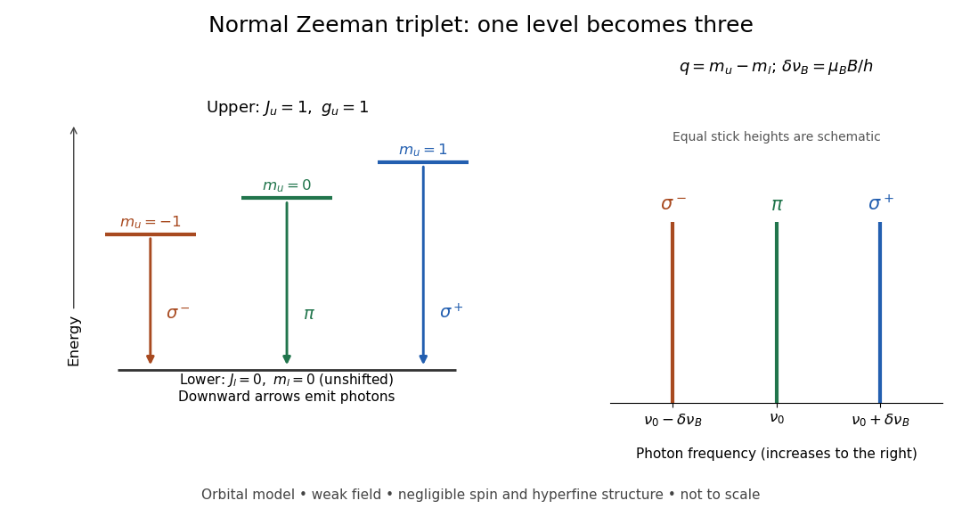
Normal Zeeman triplet from three photon transitions
. Original schematic of the ideal orbital model. The upper splitting factor is one and the lower level has zero first-order shift. Downward arrows show photon emission; the spectrum uses frequency increasing to the right. Equal stick heights are schematic and do not predict observed intensities. Details.
For an original numerical example choose and a zero-field vacuum wavelength . Using and gives . The two outer components are separated by . Differentiating the vacuum relation , with the speed of light, givesEach outer component lies about from the centre. Positive means higher frequency and shorter wavelength. Equal spacing in frequency is only approximately equal spacing in wavelength. These are calculated values for a chosen model, not historical measurements.
Viewed perpendicular to the magnetic field, the normal Zeeman effect has a component with linear polarization parallel to the magnetic field and two components polarized perpendicular to it. Along the magnetic field, vanishes and the pair has opposite circular polarizations. Pieter Zeeman described these geometry-dependent patterns in his lecture.[ref]
Light Radiation in a Magnetic Field by Pieter Zeeman. Light Radiation in a Magnetic Field, University of Maryland mirror PDF p. 3, rectilinear/circular oscillator discussion and cadmium photographs
The geometry can be derived from electric dipole radiation. Let the observation unit vector be , with measured from the magnetic field. Radiation retains only the transverse part of the oscillating electric dipole moment :For , take ; its angular light intensity factor is , so it vanishes on axis. For , use normalized complex dipoles . Their angular factors are . Projection gives circles on axis, lines at , and generally elliptical polarization between. These factors assume equal dipole magnitudes; actual line light intensities also depend on initial quantum state populations, transition strengths and collection geometry. No absolute handedness name is needed: it depends on the viewing and phase conventions.
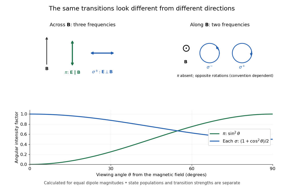
Viewing direction selects the Zeeman polarization pattern
. Original projection diagram with the magnetic field vertical. The top panels show electric-field traces as seen by transverse and axial observers. The lower plot gives calculated dipole angular factors for equal dipole magnitudes; it is not a measured spectrum or an assumption of equal state populations. Details.
A transverse polarizer can separate from even before the spectral line components are fully resolved. Along the magnetic field, a quarter-wave plate followed by a polarizer converts the two opposite circular polarizations into distinguishable linear settings. This explains why polarization analysis carried information beyond a small increase in line width.
The Landé g-factor is the dimensionless electronic magnetic splitting factor relating a level's magnetic dipole moment to its total angular momentum. In the approximation where total orbital angular momentum and total spin couple to , take the orbital factor as one and the Electron spin factor as . For ,This follows by projecting onto and using . At , it gives ; at and , it gives . A level instead has zero first-order electronic shift; the formula's zero denominator must not be used. This is distinct from the statistical weight of an atomic level , sometimes also written .
The anomalous Zeeman effect is Zeeman splitting whose pattern is not the simple orbital triplet. Spin and spin-orbit interaction make the upper and lower Landé g-factors differ. The same weak-field formula still applies when its assumptions hold: “anomalous” does not mean nonlinear in the magnetic field.
For example, take an electronic transition with and , neglecting hyperfine structure. With , the formula above gives and . The two allowed transitions have dimensionless shifts , while the transitions give . Thus there are four frequencies, even though each level contains only two magnetic quantum numbers. This is an independent worked deduction; it should not be substituted for the unresolved widths in the 1896 experiment.
Neglect hyperfine structure and use a magnetic field weak compared with the spin-orbit interaction. The sodium D doublet has transitions and . Their Landé g-factors are , and respectively. With denoting upper and lower magnetic labels, the photon shift isThe first transition has four allowed shifts ; the second has six, . The most blue-shifted component of the second is , with shift . The apparently larger shift is excluded by the electric-dipole selection rule. The level lies above , so in this weak-field model the component also has the shortest wavelength of the whole doublet. [ref]
https://physics.nist.gov/PhysRefData/Handbook/Tables/sodiumtable5.htm. NIST, Energy Levels of Neutral Sodium, ordering of the two 3p fine-structure levels
For the electronic transition, neglect hyperfine structure and use weak-field LS coupling. The Landé g-factors are and , so a transition from to shifts by .
With propagation perpendicular to the magnetic field, linear polarization parallel to the field drives the electric-dipole selection rule . The two shifts are . Perpendicular linear polarization is an equal-amplitude combination of the two field-axis circular components, driving transitions with and shifts . Each geometry therefore selects a doublet, with twice the separation in the perpendicular-polarization case. Equal line heights within a pair require equal lower-state populations and an unsaturating probe; line positions do not require that extra population assumption.
In the Paschen-Back effect, the external magnetic field interaction becomes large compared with the spin-orbit interaction that holds and coupled. Then ceases to be a good approximate quantum number; become more useful, with leading electronic shifts . In the ideal complete-decoupling limit an electric-dipole interaction preserves , so its spin contribution cancels between the levels and orbital triplet spacing can reappear. Intermediate fields require mixing the coupled states. This is a change of coupling regime, distinct from the weak-field anomalous Zeeman effect; still larger fields require additional terms beyond this linear model.
For orbital angular momentum and spin , considerThe quantum number is conserved. The stretched states with have energies . The remaining eigenvalues follow from two blocks with off-diagonal entries :The subscripts denote . For , the zero-field multiplets are at and at . Their weak-field Zeeman splitting is , with Landé g-factors and , respectively. When , the Paschen-Back effect gives approximate product states and energies . Mixing within a fixed causes an avoided crossing; different sectors can cross because the Hamiltonian does not couple them.
Articles by others on the same topic
There are currently no matching articles.