
A function between metric spaces is Lipschitz continuous if one finite number controls every change of output by the corresponding change of input:For real inputs and outputs this is . The same bound must work for every pair in the specified domain of a function. It gives a quantitative version of continuity: an input error of at most produces an output error of at most . The least possible bound is the Lipschitz constant. Lebl presents the real and metric-space definitions and their connection with uniform continuity. [ref]
Three functions show why this condition differs from differentiability. The absolute value has a corner at zero, but the reverse triangle inequality gives , so it has Lipschitz constant one on the real line. The sine is smooth and also has Lipschitz constant one: the mean value theorem and bound every secant slope. The square root is continuous on , butNo finite Lipschitz bound works on that interval. At , the ratios are . Smaller input changes near zero therefore require larger amplification factors.
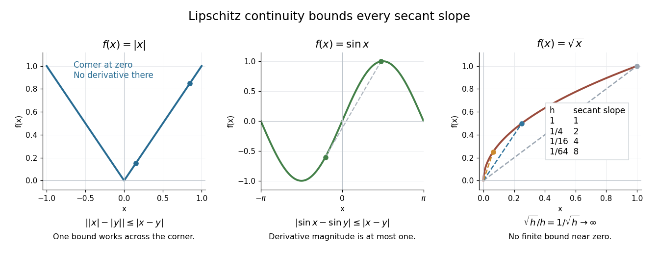
Bounded secant slopes permit a corner, while the square root needs unbounded amplification near zero
. Details. For a real function, Lipschitz continuity means that the absolute slopes of all secant lines are bounded. If the derivative exists at a point, taking a limit of those slopes gives . In the other direction, a function that is continuous on a real interval, differentiable in its interior, and satisfies there is Lipschitz continuous by the mean value theorem. The interval hypothesis matters: the theorem uses the segment connecting the two inputs.
A Lipschitz function is uniformly continuous: for , choosing input tolerance works at every point. If , the function is constant. The converse fails; the square root on is uniformly continuous, and satisfies the weaker Hölder continuity bound , without a finite Lipschitz constant. These distinctions are developed in Lebl's worked examples. [ref]
The usefulness is controlled sensitivity. Successive Lipschitz maps with bounds and have a function composition with bound , because each stage amplifies the previous distance by at most its own bound. For an ordinary differential equation, Lipschitz continuity in the unknown state is the condition that makes nearby trial solutions controllably close in the Picard-Lindelöf theorem. For incomplete data, the McShane extension theorem fills in unobserved values while preserving the same bound. This one inequality connects error estimates, uniqueness, and interpolation.


Lipschitz continuity is a condition that describes how a function behaves with respect to changes in its input values.
New to topics? Read the docs here!